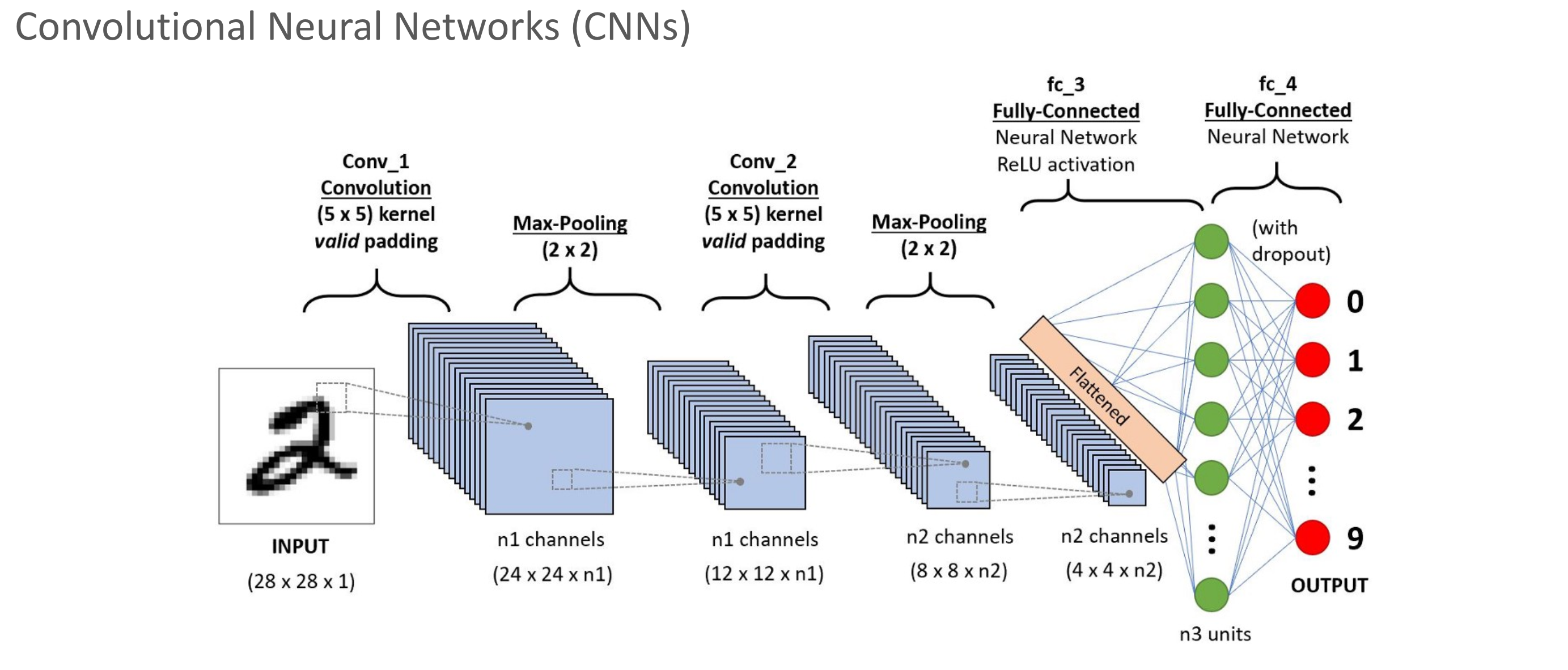
CNN
Summary
Vision 계열 대표 base 모델이자 architecture.
2012년 IMAGENET Challenge에서 AlexNet이 SOTA 달성하며 알림.
가장 핵심은 convolution(정확히는 cross-correlation) 연산을 수행하는 filter.
key: “feature를 filter로 추출하자.”
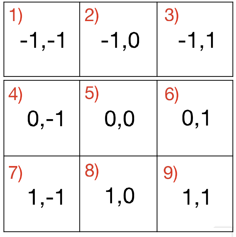
Convolution vs Cross-Correlation
일반적인 DL context에서 사용되는 연산은 모두 cross-correlation이다.
filter를 target matrix에 적용할 때에, entry 순서 맞춰서 적용하는 것이 cross-correlation.
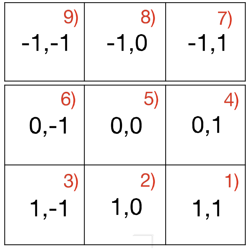
convolution은 순서를 바꿔야 함.→ 이로 인해 convolution의 경우, associative property 지님.
Multi column
Cross Correlation
Convolution
Before the CNN
FC layers
NOTE
형태인 fc layer는 output으로 score를 뱉어냄.
pixel space에서 projection한 걸로 볼 수도.
이걸 visualization 해보면, 클래스 별 template을 가질 수도 있고 그럼.
Feature Representation
- 직접 hand tuning하여 feature를 정의하고 detect.
- DL 이전에 꽤 많이 사용됨.
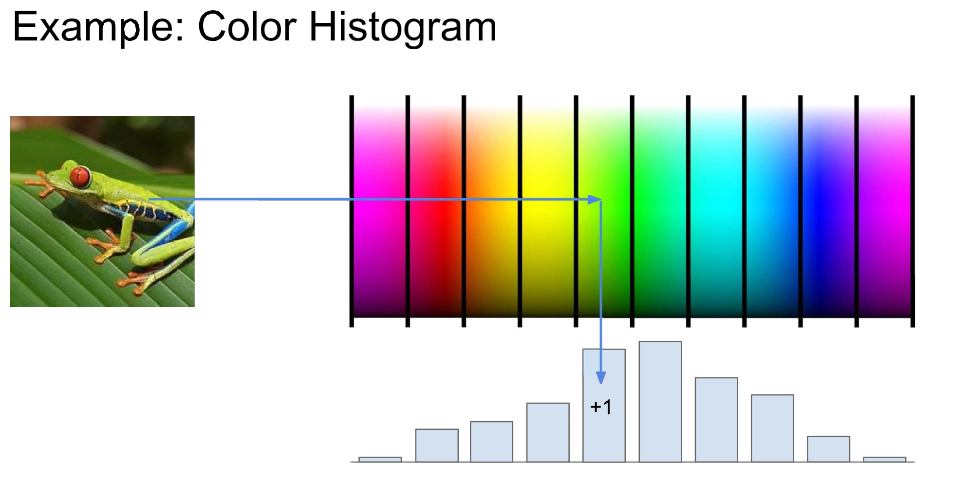
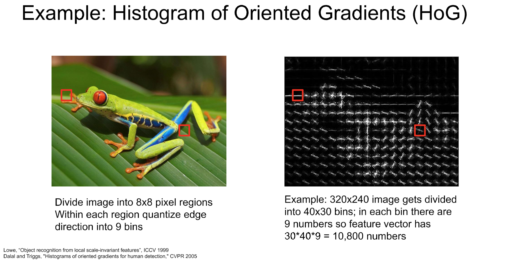
Color Histogram → HoG
NOTE
이렇게 frog의 feature인 color를 다룬다던지
color gradient 즉, 색이 급변하는 것을 detect해서 edge로 인식하게 coding.BoW(Bag of Words)
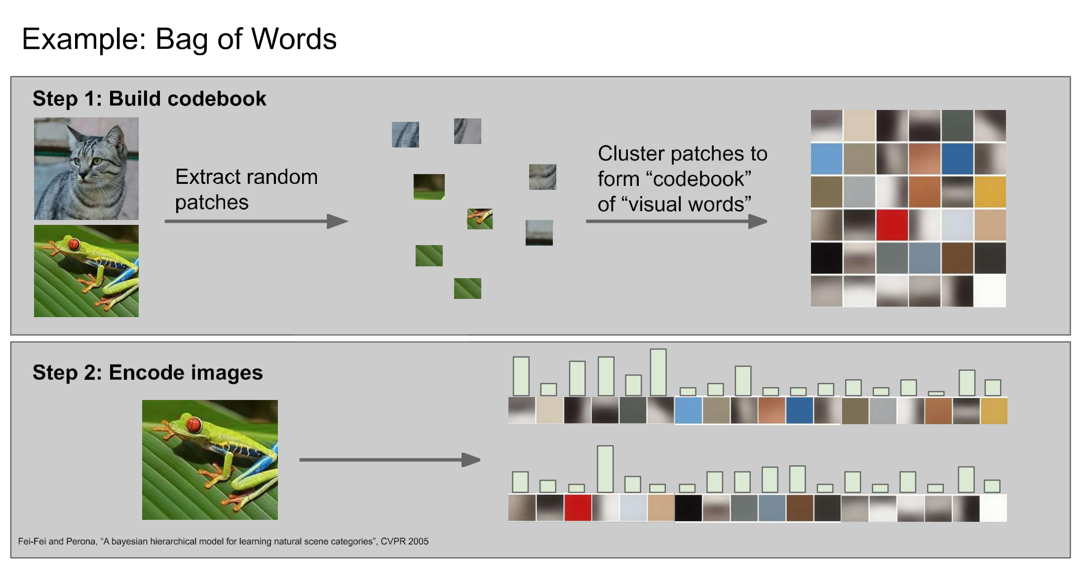
NOTE
- NLP에서도 과거 자주 사용되던 방법.
step1. dictionary 정의
- 사전(codebook)을 만들기 위해 사진에서 random하게 patch 만들고 원본의 label을 붙여서 만듦.
step2. image encode
- dictionary 활용해서 이미지들을 encoding
Summary
Feature 접근이랑 비교해보면, feature extracting을 모델이 직접하게 한 데에 의의가 있다.(ConvNet)
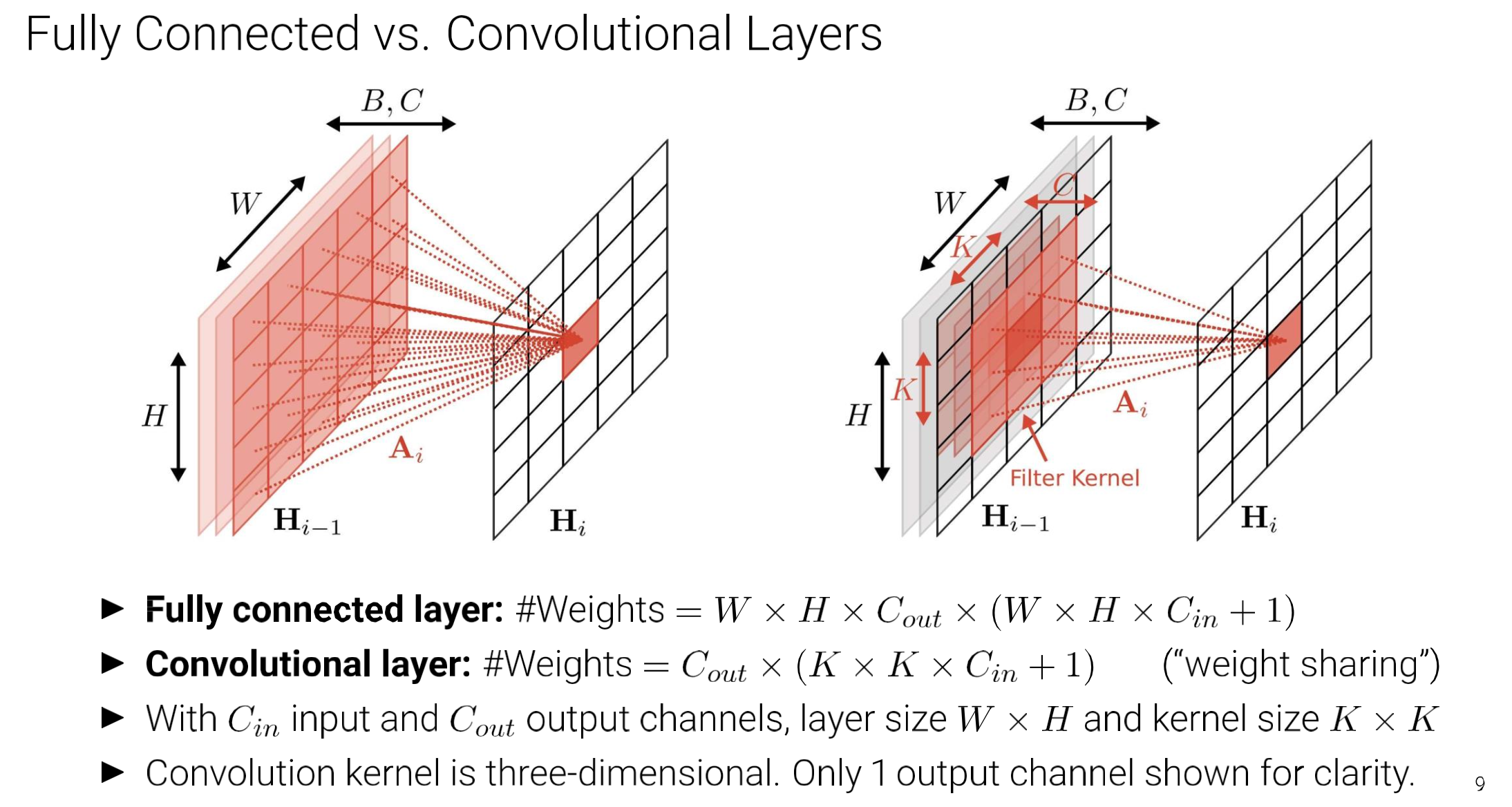
FC layers vs Convolution layers
Note
- “weight sharing”
- 1 : bias
Main Concepts of CNN
Important
- Sparse-connectivity: FC는 말 그대로 하나의 output value가 이전 layer output의 weighted-sum 형태로 들어가니, 하나의 activation에 관여하는 값들이 너무 많음. 반면, CNN은 sparse하게 locality를 잘 살린 architecture하고 볼 수 있음.
- Parameter-sharing: filter가 translation하면서 convolution 연산하니, parameter를 공유하는 효과
- Many layers: 여러 filter를 한 번에 사용하여 pattern인식에 수월.
Question
filter끼리 안 비슷해질라나?
Question
Is CNN only for img? → Nope. Also can be performed in audio area.
CNN in audio detection(ex)
Todo
- task: 위 spectrum을 가지고 ‘welcome’ 발화 부분 segmentation
by using MLP...
이렃게 trivial 하게 전 영역을 MLP하면 되겠지만, 문제는
이렇게 데이터가 주어진다면,
- 위 사진의 데이터로만 학습하면 target이 다른 위치에 있는 즉, 아래 사진의 경우를 예측하기 힘들다.
- 또한, NN의 size도 크고, 연산량이 너무 많이 필요할 뿐더러, 다른 위치에 target이 등장하는 데이터가 발생하면 재학습해야 한다.
Important
결국 우리가 원하는 건, translation에 무관하게 잘 예측하는 분류기!
→ translation에 무관하게 : Shift InvarianceScan
원본 링크Summary
작은 MLP를 window크기 만큼 움직이며, scan.
이후 max 통과 시키면 있었는지 여부는 확인할 수 있겠지.
아님 task에 따라 max 대신, softmax, MLP 등을 붙일수도 있겠지Example
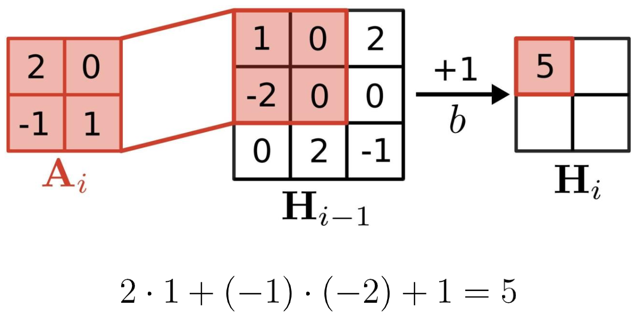
- bias 잊지 말 것.
- element-wise 연산
- Low-rank~ 는 구현 파트에서 다룸.
Conv-Layer
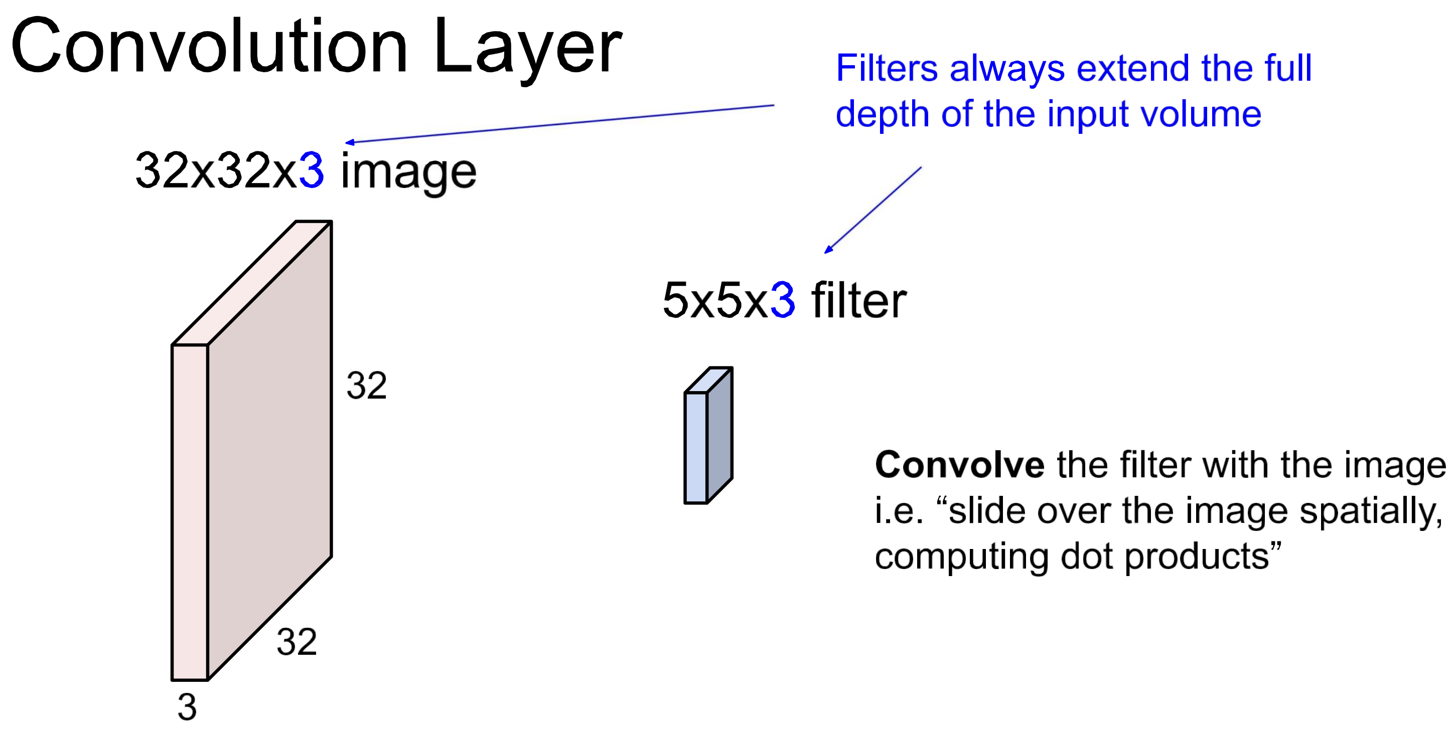
Filter size
Conv layer에서는 마지막 차원을 일치시켜야 함. (filter_depth)
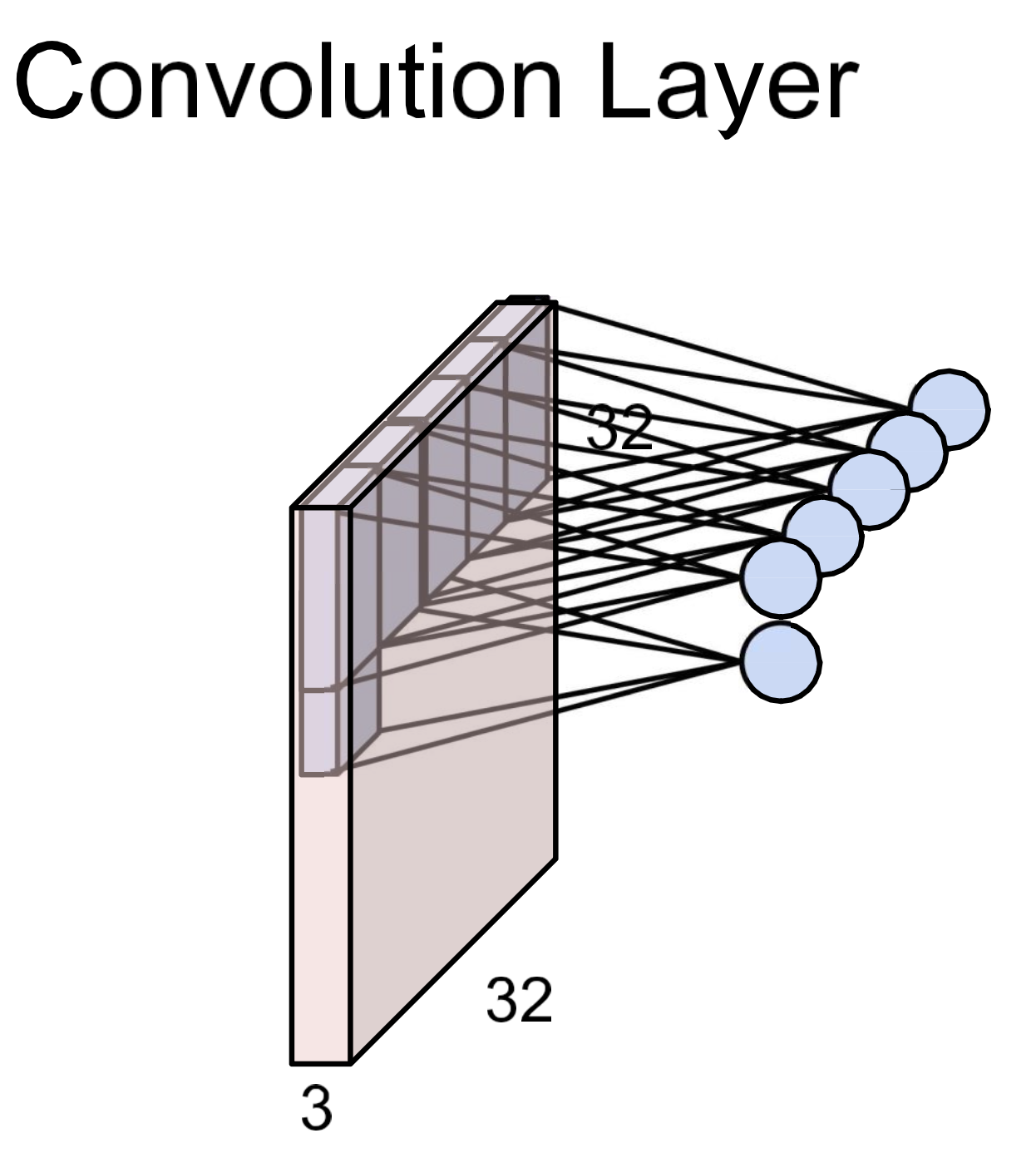
Activations
결국 한 번의 convolution 연산 output은 scalar 하니이고 이걸 이동하며(sliding) 모아서 output 전체를 구성.
- output을 feature map이라고 함.
- 한 번의 convolution 연산에 사용되는 input 영역을 receptive field라 함.
- weight sharing
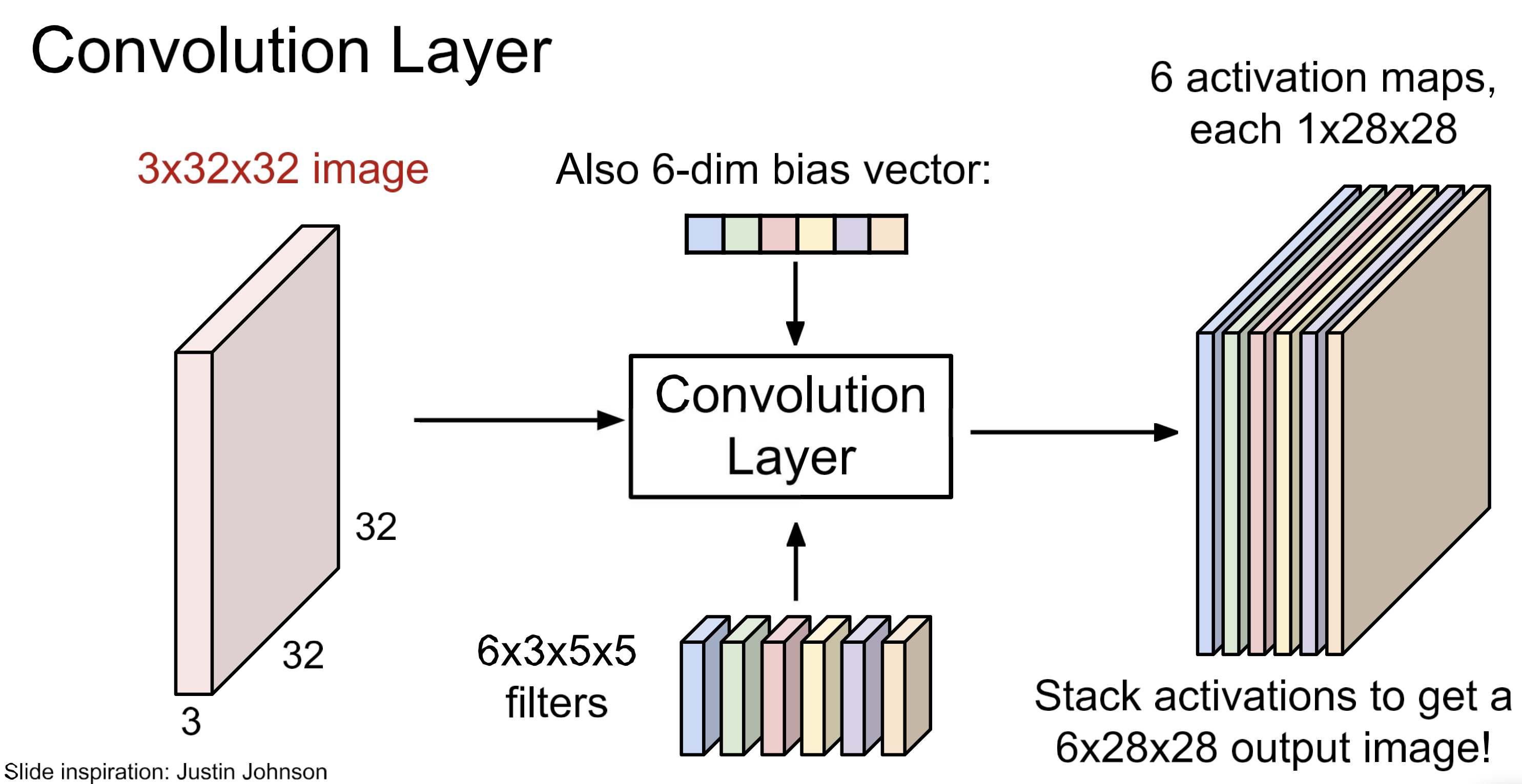
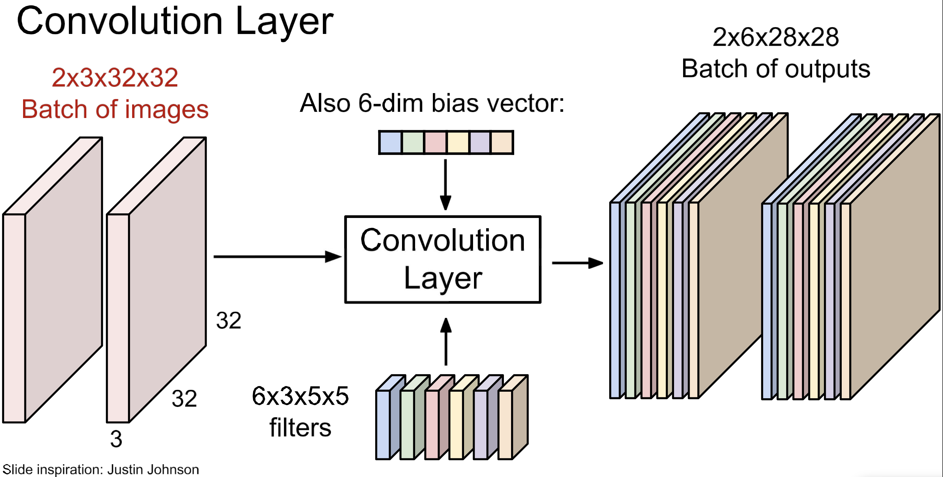
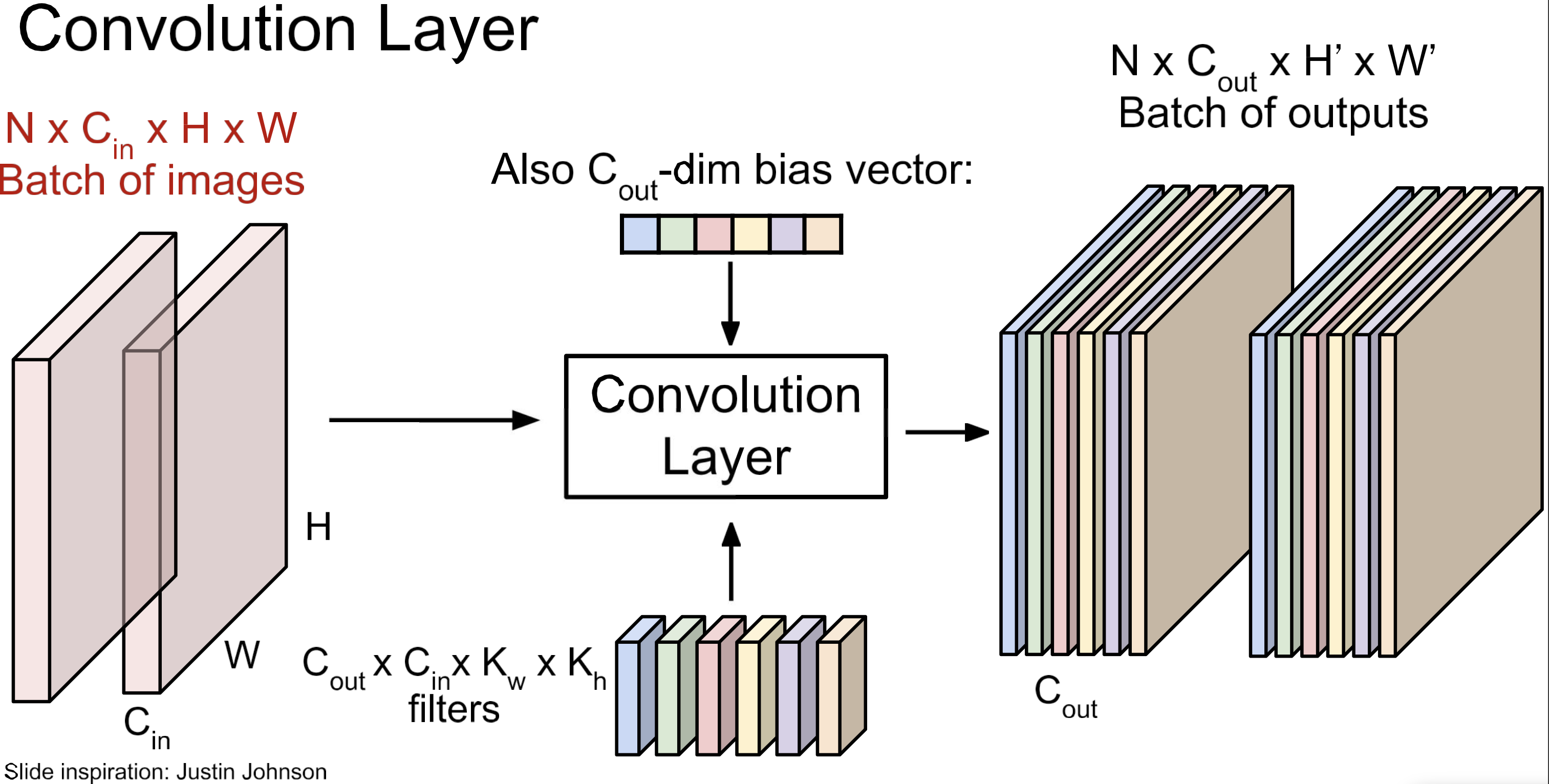
Layer overview
filter(kernel)이 여러 개이면, 위 그림과 같은 구조.
각 kernel 별 bias 가 하나씩. 즉, bias의 개수 = kernel의 개수
batch 처리까지해서 본 view.
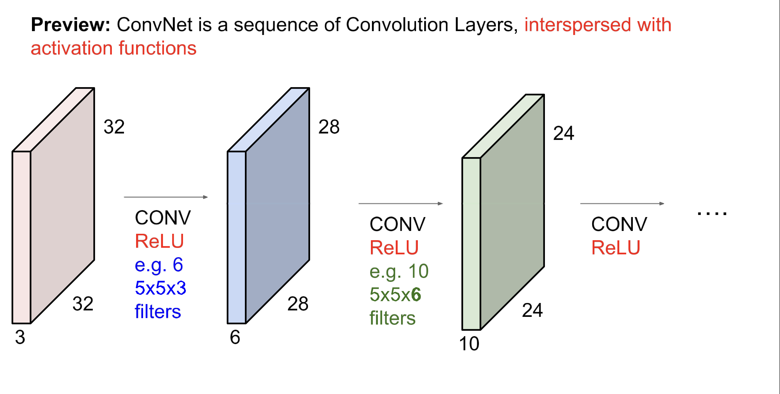
문자화해서보면 위 처럼. 이게 Conv Layer. 이제 이 layer를 여러개 쌓고 중간에 activation function을 넣어주면,
ConvNetWhat do Filters learn?
Multi column
Linear classifier
One template per class
MLP
Bank of whole-image template
AlexNet
First layer conv filter : local image templates(edges, opposing color)
AlexNet: 64 filters(3x11x11)
Feature map size
NOTE
Example
Input size: 32 x 32 x 3
Kernel : 10 per each 5x5 with stride=1, padding=2
output size?
(32-5+2x2)/1+1 = 32 (output size)
32x32x10 (output size per channel)
Number of parameters in this layer?
10 x (5 x 5 x 3 + 1)
760
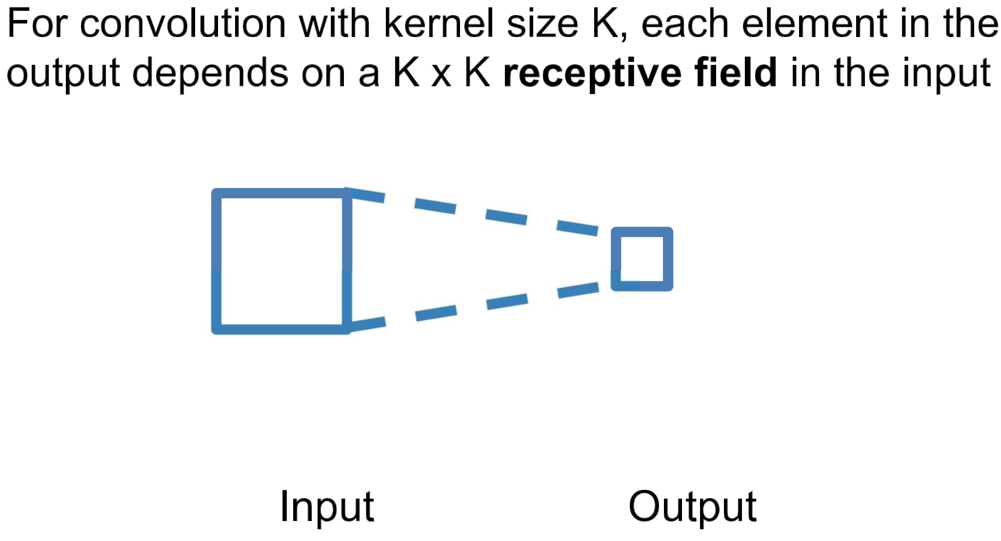
Receptive Fields
NOTE
한 번의 convolution 연산 시 사용되는 Input의 regieon
Warning
“receptive field in the input”
“receptive field in the previous layer”Architecture
Components
Summary
- Conv Layer
- Pooling Layer
- FC Layer
- Normalization Layer
- Activation Function
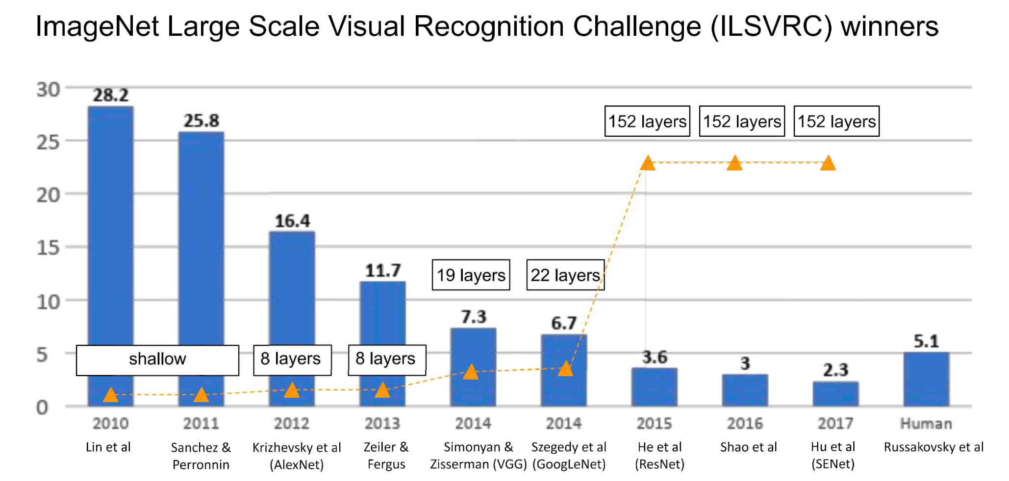
Case Study
Info
ILSVRC(ImageNet Large Scale Visual Recognition Challenge)
- image classification 대회
- 향후 kaggle로 흡수됨.
원본 링크
- AlexNet
- ZFNet
- VGGNet
- GoogLeNet
- ResNet
- SENet
- DenseNet
- Deep Residual Networks
- Wide Residual Network
- MobileNets
- Neural Architecture Search with Reinforcement Learning(NAS)
- EfficientNet
/../../../../../AI/Concepts/Architectures/CNN/assets/audio-spectrogram.png)
/../../../../../AI/Concepts/Architectures/CNN/assets/audio-seg-mlp.png)
/../../../../../AI/Concepts/Architectures/CNN/assets/audio-seg-mlp-prob.png)
/../../../../../AI/Concepts/assets/shift-invariance-soln-scan.png)