Computation graphs

How to compute gradients for our model?

결국 하려는 것은 모델의 파라미터를 개발자들이 manual 하게 define 하는 것이 아니라, model 이 learning하게 하고 싶은 것. 그러기 위해서는 데이터를 잘 설명하는 parameter를 tuning 해야하는 거고.

→ 파라미터를 업데이트 해야하나? → Loss를 기준으로
→ 파라미터를 어디 방향으로 얼마만큼 update? : Loss의 gradient를 사용해서.
결국, $\frac{\partial L}{\partial W}$ 값이 필요하다

Approach 2: Derive ${\nabla }_{W}L$ on paper : analytic (Bad Idea)

Problem : Very tedious. Lots of matrix calculus, need lots of paper.

Problem: What if we want to change the loss function?
→ re-calculate,,

Problem: Not feasible for every complex models!

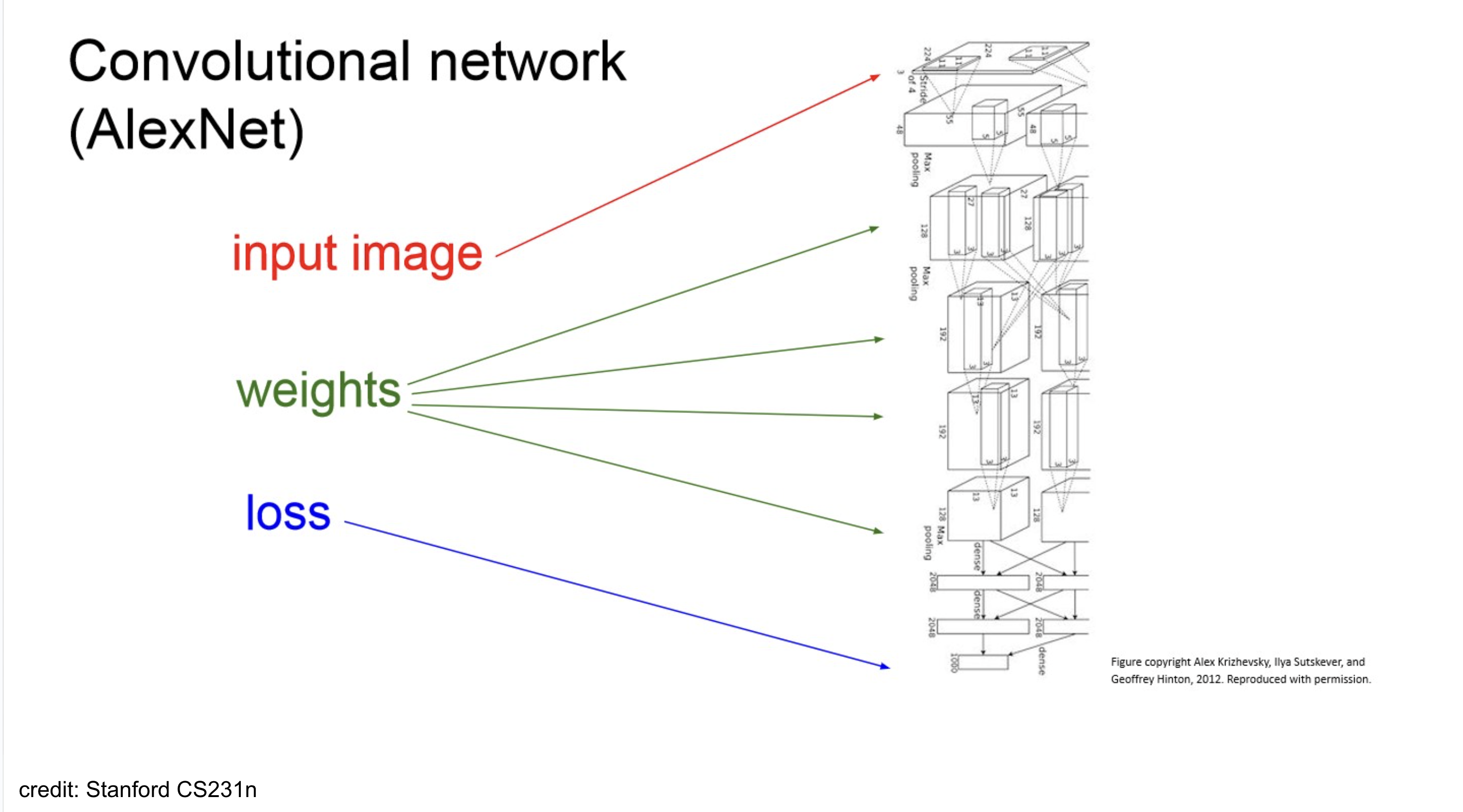
Multi column

example-AlexNet

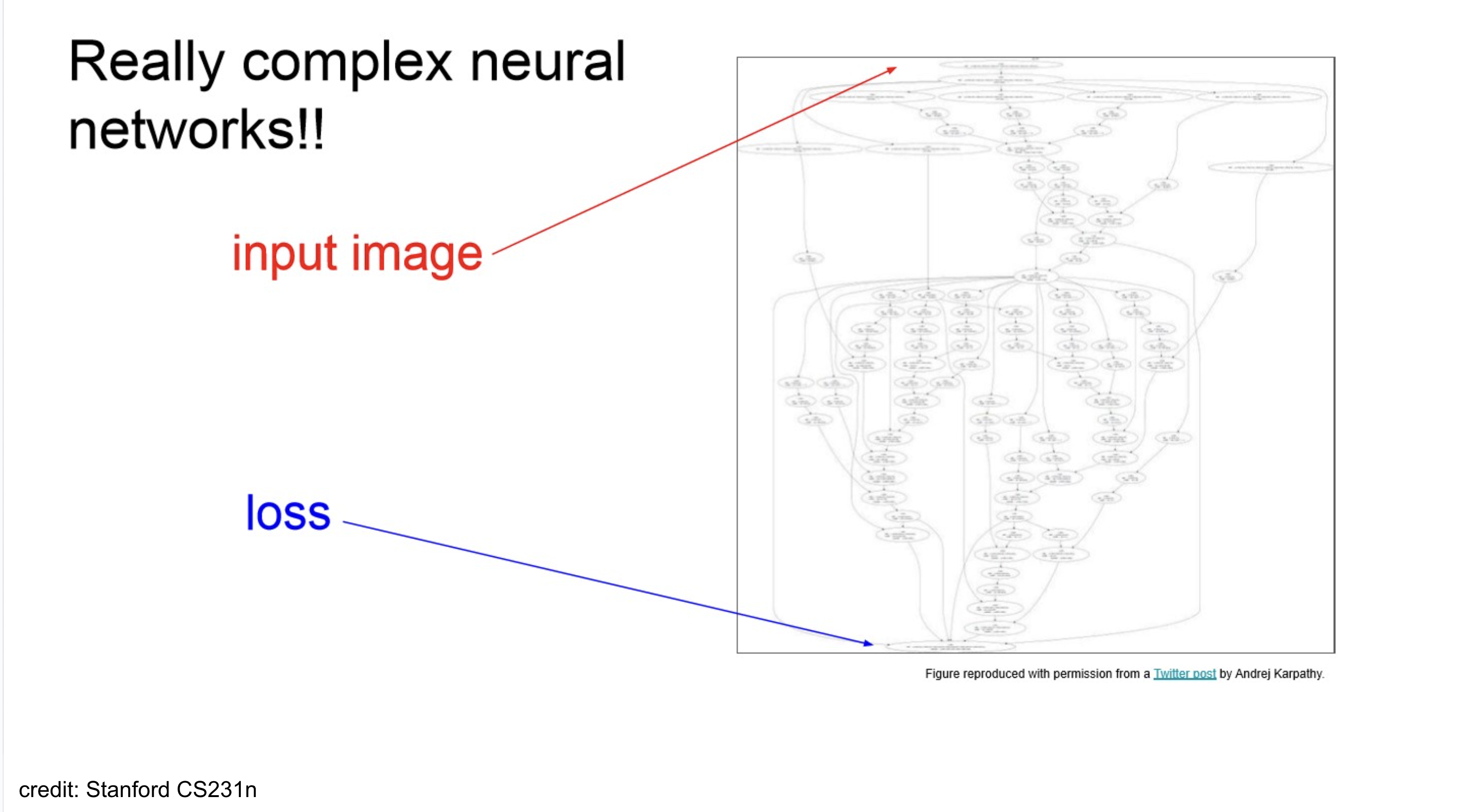
example-Neural Turing Machine

Approach 2: Computational Graph + Backpropagations

Problem : Very tedious. Lots of matrix calculus, need lots of paper.

Problem: What if we want to change the loss function?
→ re-calculate,,

Problem: Not feasible for every complex models!

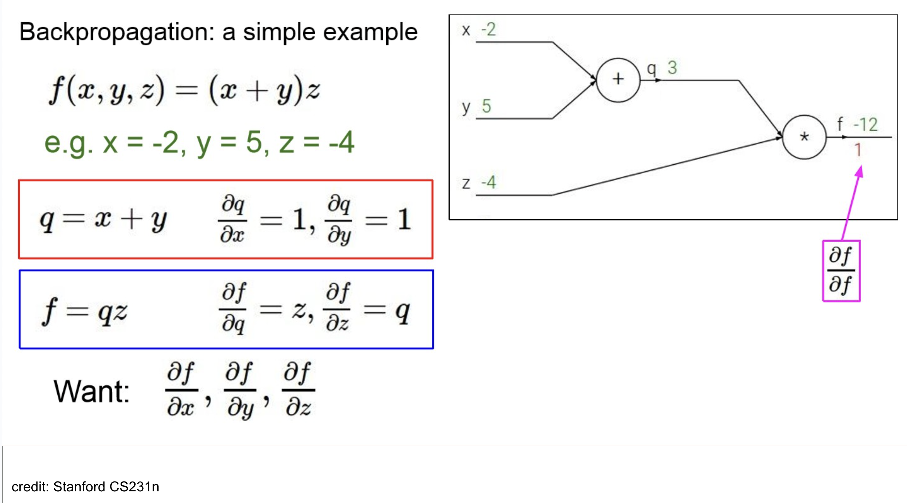
Computational Graph

그래프화 해서 Visualize!

• green line: forward pass
• red: backward

쭉 계산해보면 위와 같다.
보이는 것처럼 모델이 깊어지면,(multi-layer) chain-Rule을 사용해야 할 만함.

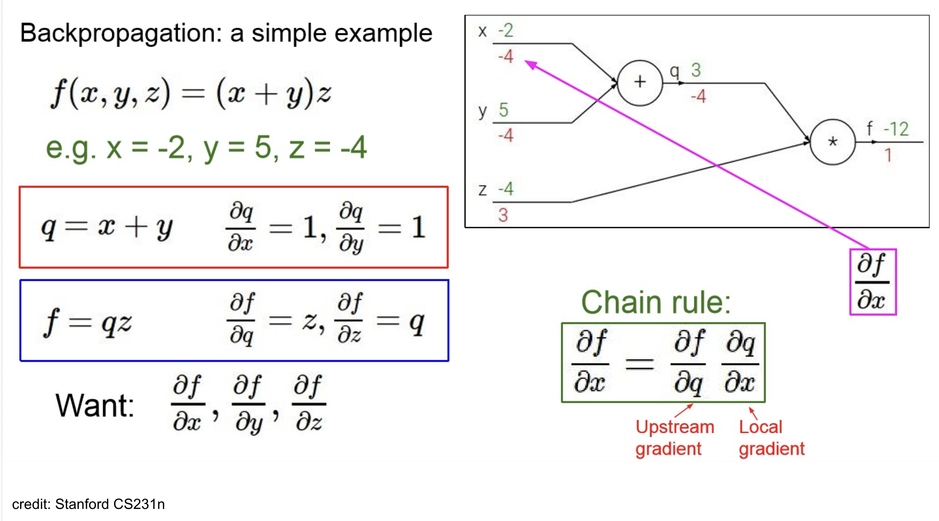
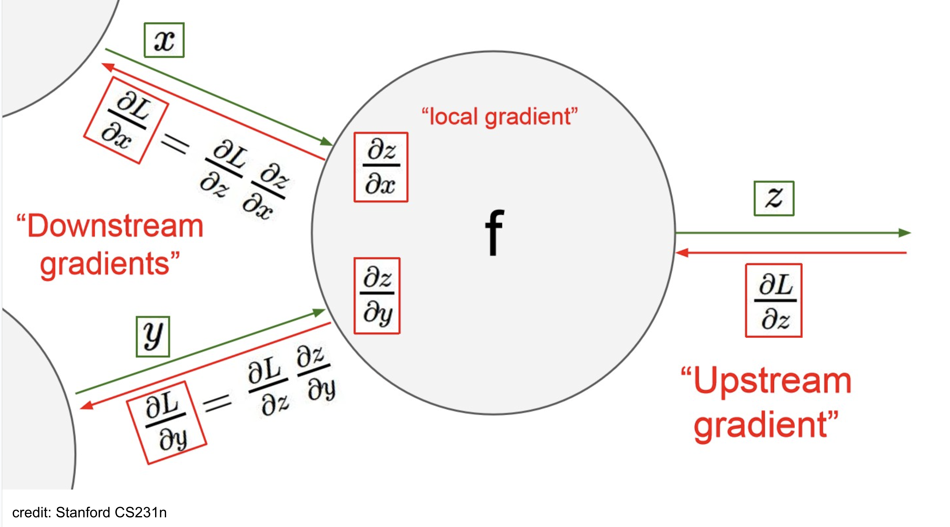
Terminology

아래 용도들은 node 기준으로 define됨.

• upstream-gradient: node로 들어오는 gradient 값. (backward-pass direction)
• local-gradient: 현재 node에서 계산하는 gradient.
• downstream-gradient: node에서 나가는 gradient 값. (upstream* local) gradient (by chain-rule)

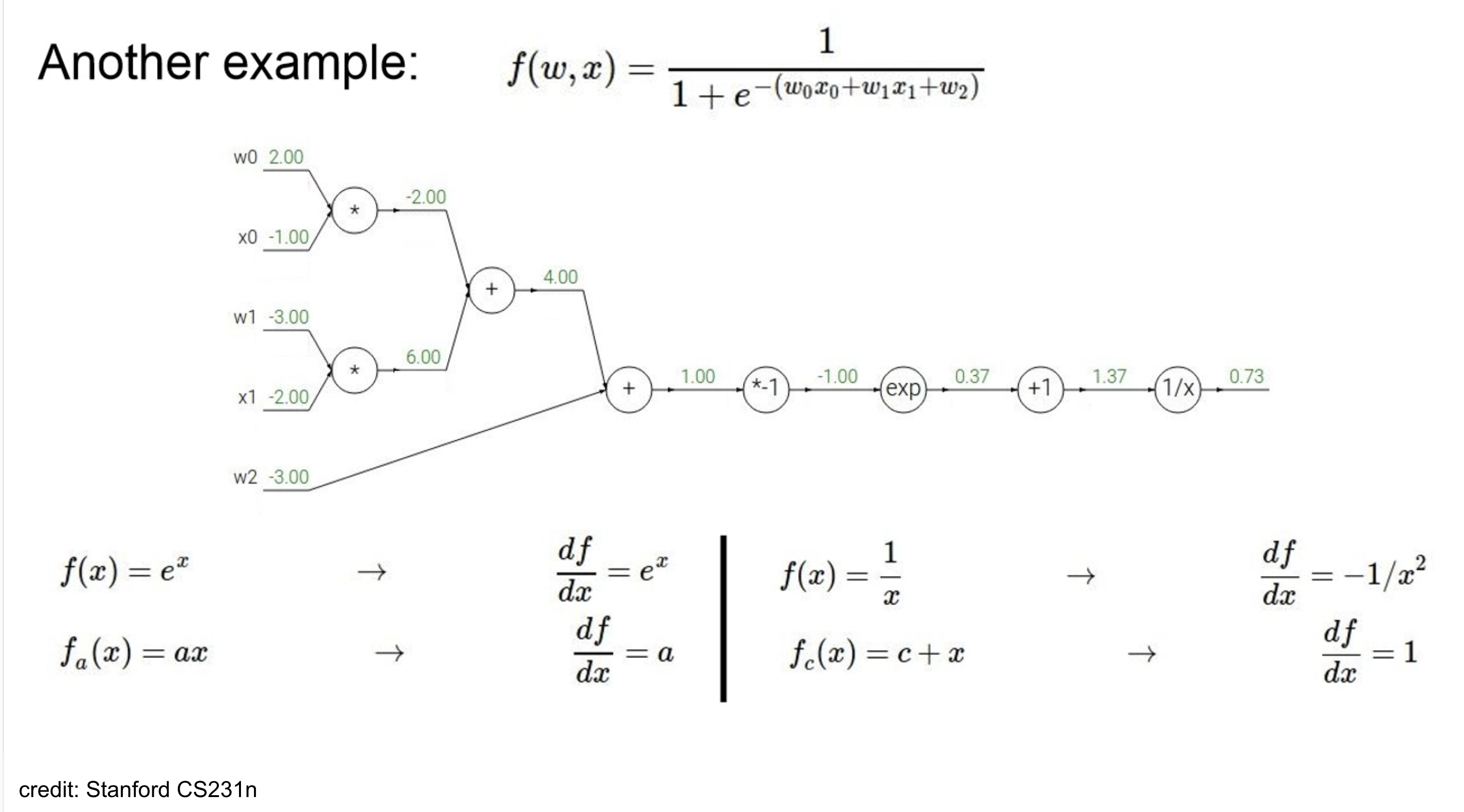
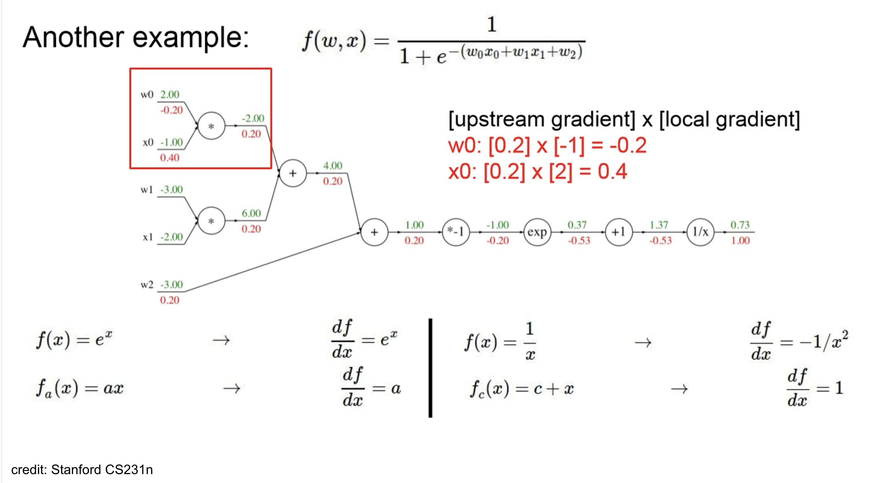
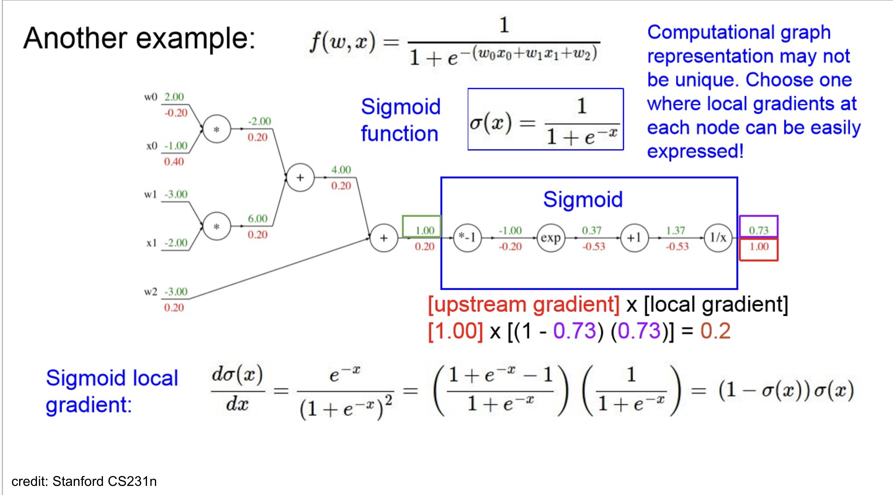
Computational Graph Calculation Ex

$\frac{1}{x}$ node 기준으로 보자면,

• upstream gradient는 1.00 ($\frac{dL}{dL}=1.0$)
• local gradient는 $\frac{dL}{df}$ where $f(x)=\frac{1}{x}$
  따라서, downstream gradient는
• $\frac{dL}{df}=\frac{dL}{dL}\frac{dL}{df}$ (by chain-rule) $=(1.0)(\frac{-1}{1.37^2})=-0.53$

쭉 하다보면 위와 같고,
잘 보면 activation이 sigmoid인데, 효율적으로 생각해보면 이를 하나의 node로 처리할 수 있다.
$\frac{d}{dx}\sigma (x)=\frac{d}{dx}(\frac{1}{1+e^{-x}})=\frac{e^{-x}}{(1+e^{-x}{)}^2}=\frac{1}{1+e^{-x}}\frac{e^{-x}}{1+e^{-x}}$
$=\sigma (x)(1-\sigma (x))$

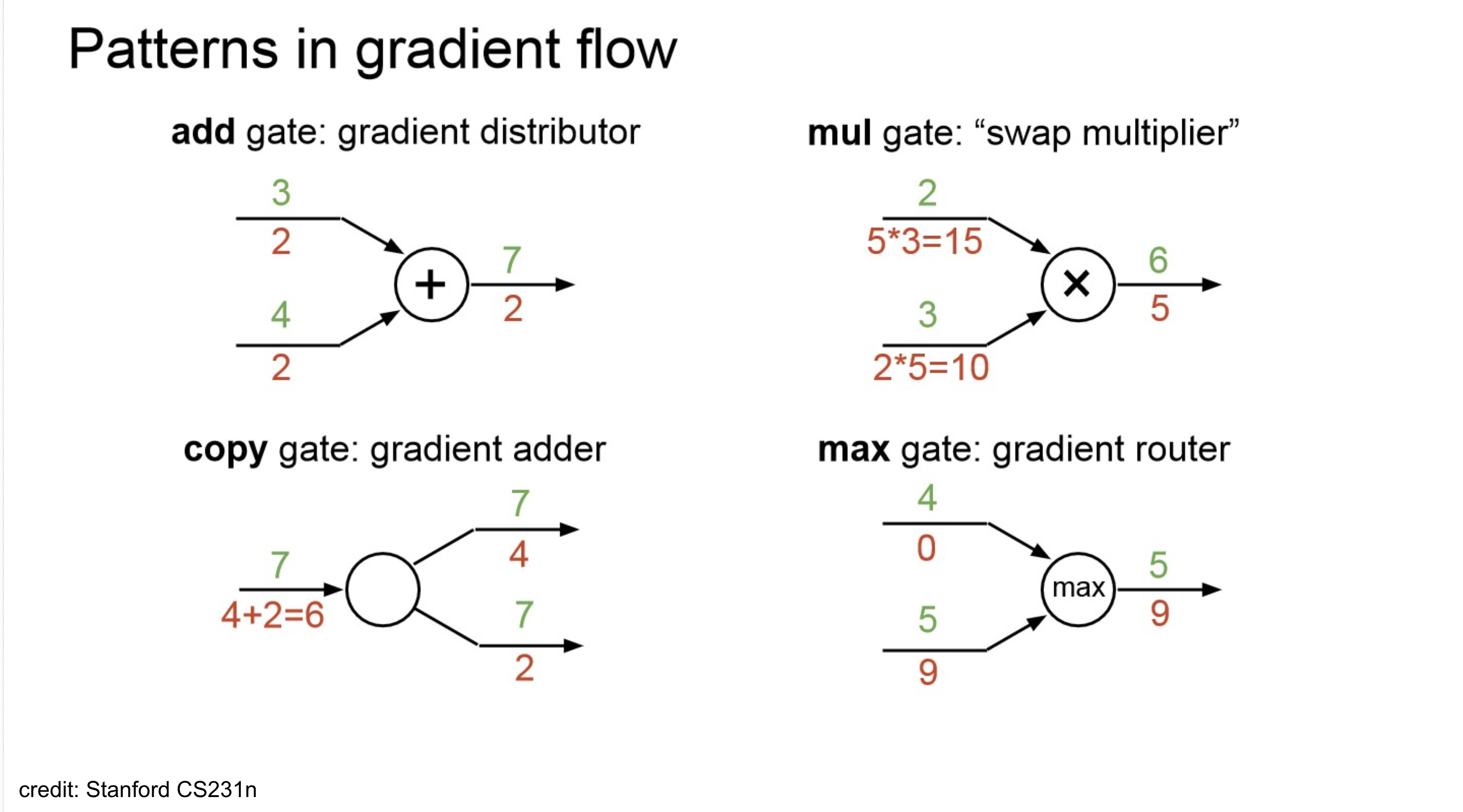
Gradient Flow Patterns

• add-gate(gradient distributor): back node에서 온 upstream이 그대로 downstream-gradient가 됨.
• copy-gate(gradient adder): gradient가 cumulative 됨.
• mul-gate(swap-multiplier): partial derivative 특성 상 미분 대상이 아닌 나머지는 상수 취급하는 성질이 적용. 나머지 노드에 대한 곱이 적용되서 downstream-gradient가 됨.
• max-gate(gradient router): forward pass에서 survive한 node로 backward가 흘러감.

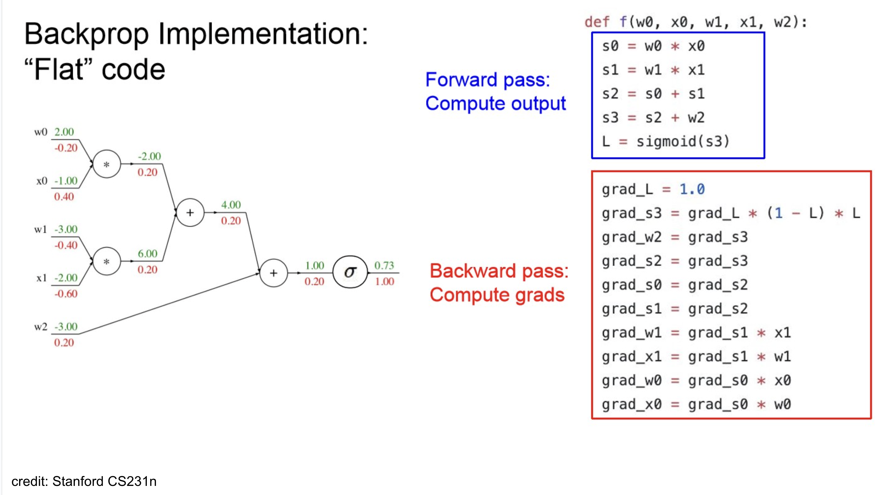
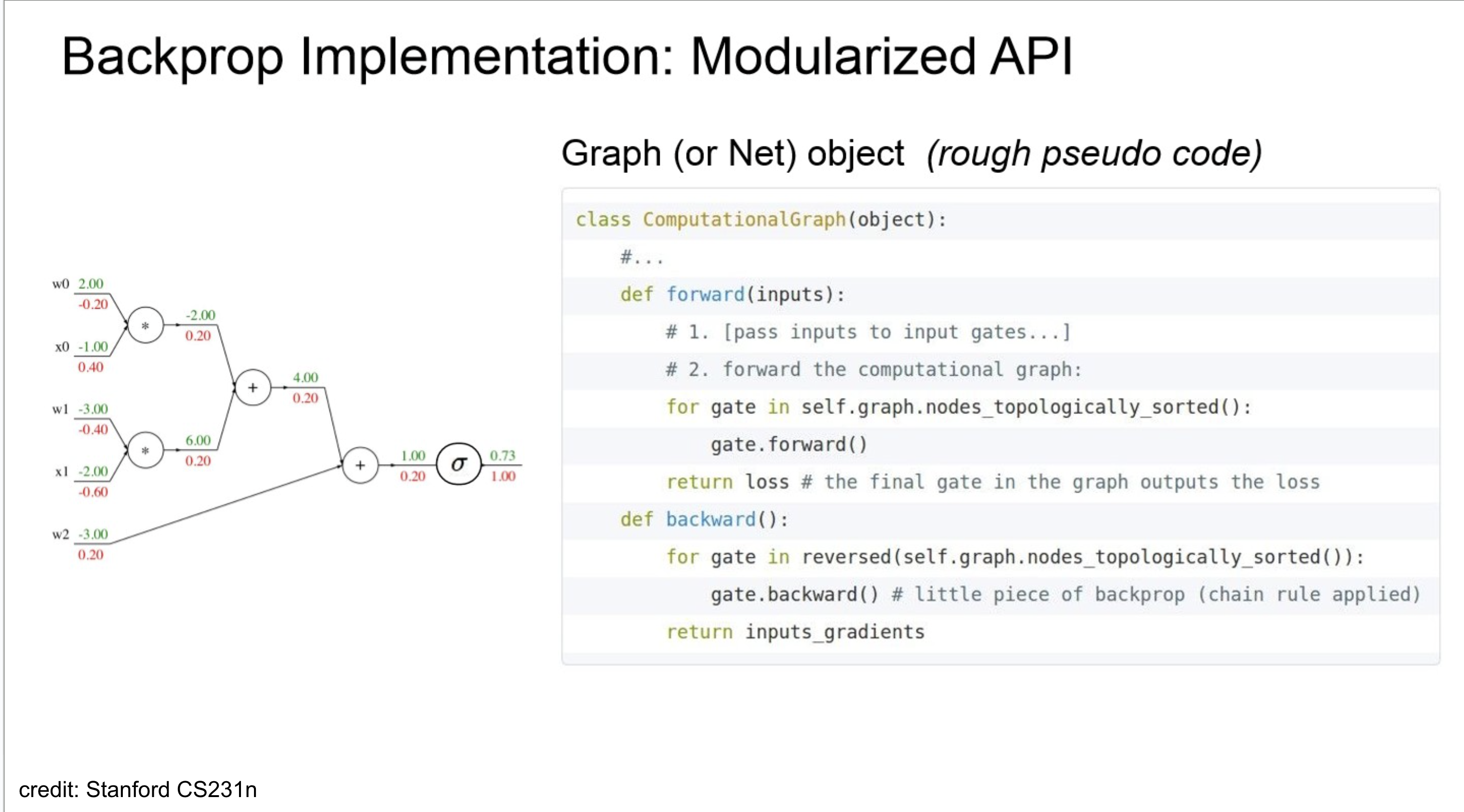
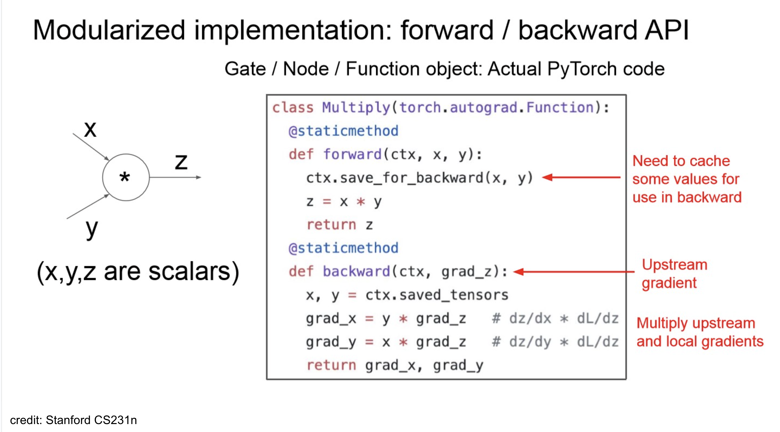
Backpropagation Implementation

• 재밌게 볼만한 점은 topological-sort?
  • 여러 연산이 섞여 있어서 순서 고려 안해주면, backward pass 시 꼬임.

• 또한, backward 시 chain-rule을 사용하니, forward에서 나온 일부 output 값들이 필요하니 중간중간 caching 해두는 부분 존재.

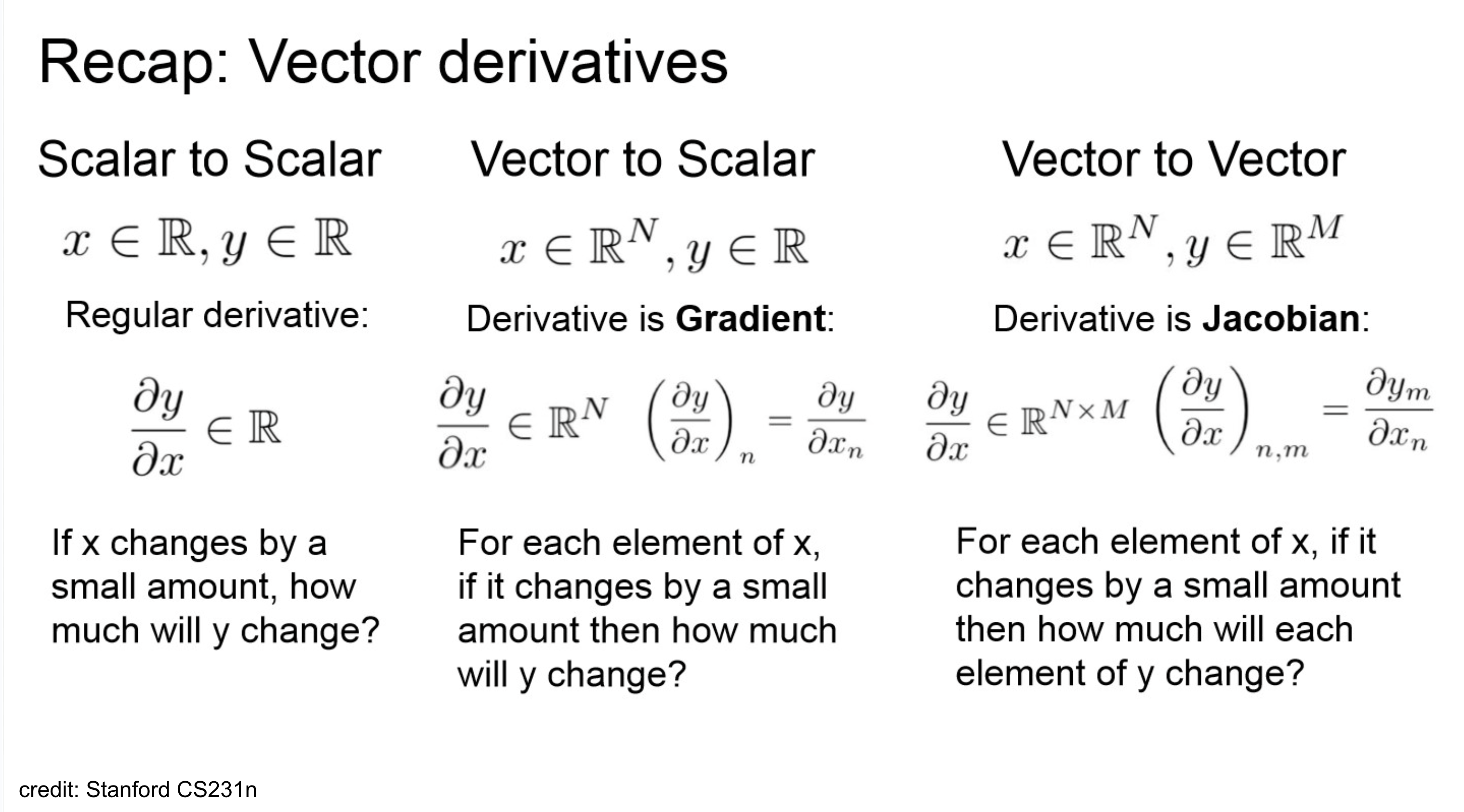
Recap: Vector derivatives

$\text{Loss is always a scalar!}$

• 하나 더 추가하면, Hessian도 구분할 줄 알아야 하고, Hessian은 2계도 미분이라는 점.

Backward pass with Vectors

“Gradients of variables wrt loss have the same dims as the original variable.”
→ debugging용으로 아주 좋지..

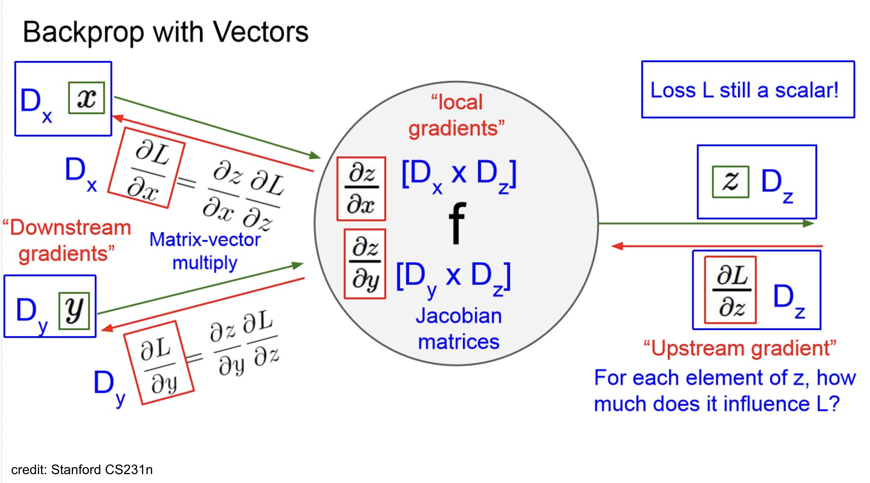
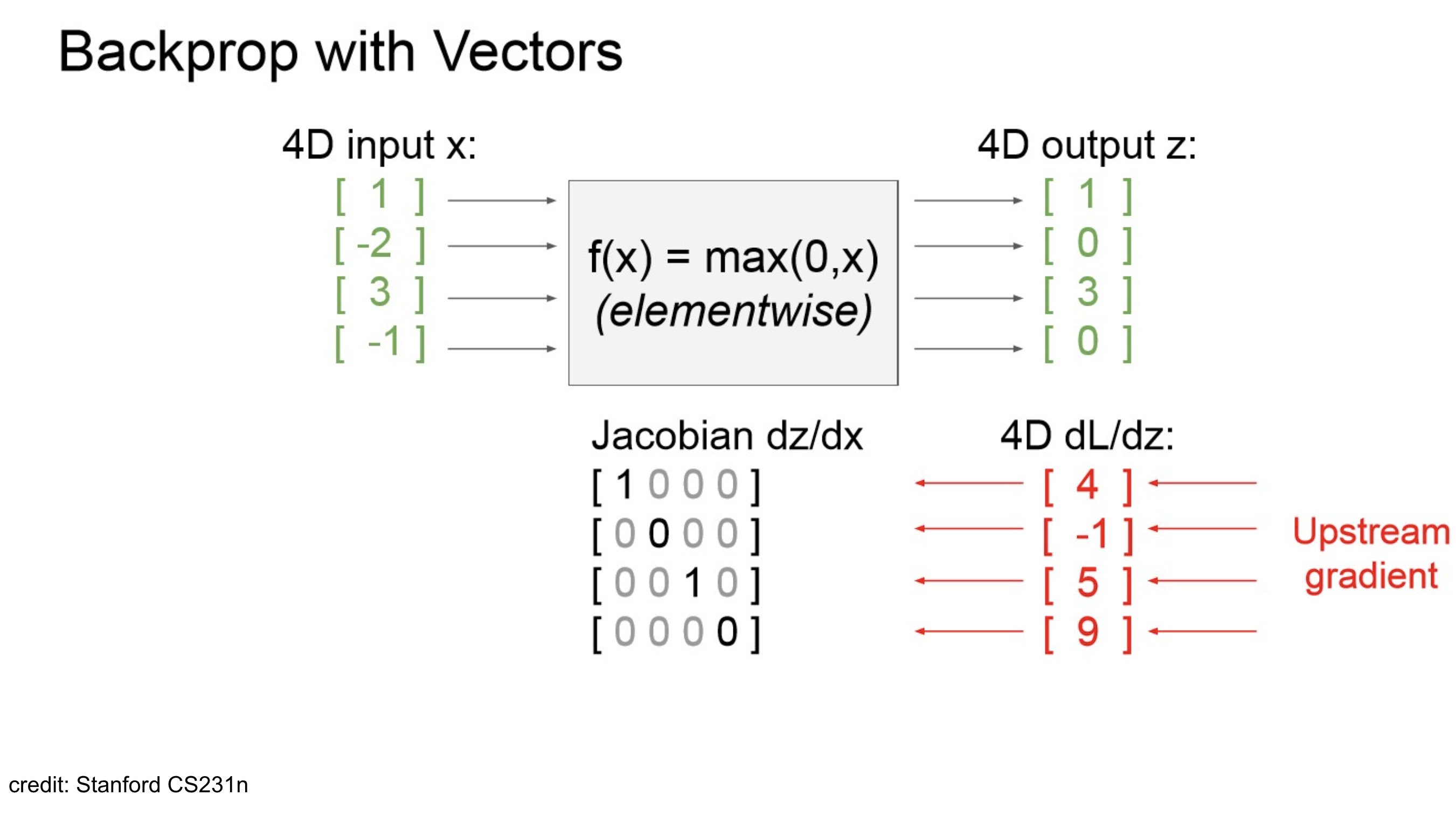
Backprops → Jacobian

• 현재 상황이 4d vector를 ReLU 통과 시킨 건데, 결과된 결과를 이렇게 생각해보자.
  Let input vector x as a

x_0 \\ x_1 \\ x_2 \\ x_3 \end{bmatrix} = \begin{bmatrix} 1 \\ -2 \\ 3 \\ -1 \end{bmatrix} $$ $$ReLU(\mathrm{x}) = ReLU(\begin{bmatrix} x_0 \\ x_1 \\ x_2 \\ x_3 \\ \end{bmatrix}) = \begin{bmatrix} ReLU(x_0) \\ ReLU(x_1) \\ ReLU(x_2) \\ ReLU(x_3) \\ \end{bmatrix} = \begin{bmatrix} 1 \\ 0 \\ 3 \\ 0 \\ \end{bmatrix}

여기서 Jacobian $\frac{dz}{dx}$는 아래와 같이 계산된다.

$$\left[\begin{array}{cccc}\frac{\partial }{\partial x_0}ReLU(x_0)& \frac{\partial }{\partial x_0}ReLU(x_1)& \frac{\partial }{\partial x_0}ReLU(x_2)& \frac{\partial }{\partial x_0}ReLU(x_3)\\ \frac{\partial }{\partial x_1}ReLU(x_0)& \frac{\partial }{\partial x_1}ReLU(x_1)& \frac{\partial }{\partial x_1}ReLU(x_2)& \frac{\partial }{\partial x_1}ReLU(x_3)\\ \frac{\partial }{\partial x_2}ReLU(x_0)& \frac{\partial }{\partial x_2}ReLU(x_1)& \frac{\partial }{\partial x_2}ReLU(x_2)& \frac{\partial }{\partial x_2}ReLU(x_3)\\ \frac{\partial }{\partial x_3}ReLU(x_0)& \frac{\partial }{\partial x_3}ReLU(x_1)& \frac{\partial }{\partial x_3}ReLU(x_2)& \frac{\partial }{\partial x_3}ReLU(x_3)\end{array}\right]$$

즉, diagonal entry만 살아남을 수 있는 구조이고, activation function이 ReLU이니, 0보다 큰 곳에서만 1

1 & 0 & 0 & 0 \\ 0 & 0 & 0 & 0 \\ 0 & 0 & 1 & 0 \\ 0 & 0 & 0 & 0 \\ \end{bmatrix}$$ - Jacobian is sparse: off-diagonal entries always zero! - Never explicit form Jacobian -- instead use implicit multiplication