Numpy

Numpy

python에서 행렬 및 수에 관련된 자료를 다루기 위해 만들어진 lib.
수치 관련 연산에서 빠르다는 게 가장 큰 장점.

Numpy basics

---

다음과 같은 vector inner product function을 구현해 보자.

$z={\sum }_i{x}_i{w}_i=x_1{w}_1+x_1{w}_2+\cdots +x_n{w}_n=x^{\mathrm{T}}w$

def loop_approach(x: list[float], w:list[float]) -> float:
	z = 0.
 
	if len(x) != len(w):
		raise ValueError("x and w must have the same length")
 
  for idx in range(len(x)):
	  z += x[idx] * w[idx]
 
	return z

%timeit

시간을 측정해주는? magic keyword??

이는 numpy lib에서 dot() method로 구현되는데, 여기서 decorator를 사용하고 안 하고의 차이는?

결론적으로, x @ y에서 @는 데코레이터는 아니다. @는 python의 행렬 곱 전용 연산자(operator)이다.

일단 사용해보면, matmul 속도는 압도적으로 numpy 사용시 좋은데 뭘 구현했길래 이러한 속도 차이가..?

Broadcasting (@=matmul vs dot)

두 method 간 broadcasting 방법이 다르다고 한다.

• N차원(스택) 처리: @/matmul은 스택 차원 브로드캐스팅 지원
• dot은 마지막 축 × 끝에서 두 번째 축에 대한 합산 규칙(브로드캐스팅 방식이 다름)

python decorator

??

np.array(array-Like data)

array-like한 자료를 np.ndarray 형으로 변환해주는 method.
최대 32차원까지 문제 없이 지원해줌.
2차원일 경우, axis0는 col, axis1은 row 방향이다.
default dtype은 int64
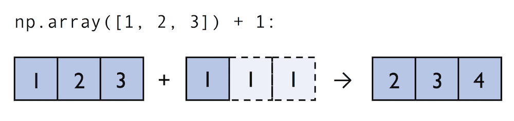
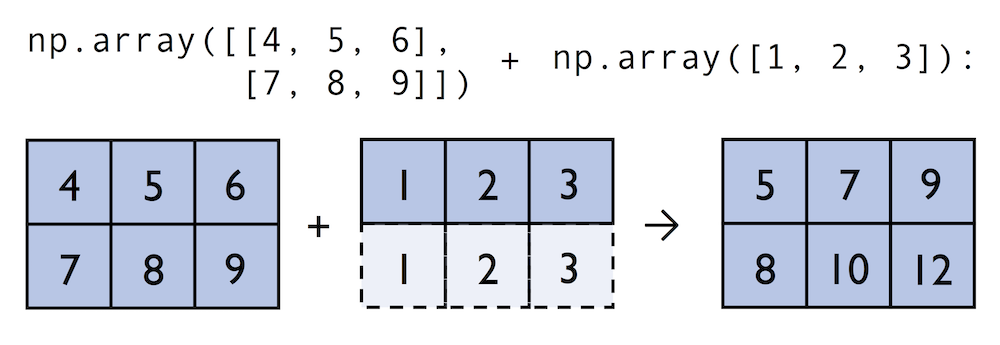
생성된 ndarray 형에는 +, -, x, / 같은 연산자들이 auro-broadcasting 되어 적용됨.

np.array().dtype

np.adarray()의 atribute로 저장된 하나하나의 dtype을 반환

np.array().astype()

np.adarray()의 dtype은 변환해주는 method.

np.array().ndim

np.adarray()의 dim 수를 반환하는 attribute

np.array().shape()

np.adarray()의 각 dim 별 사이즈를 반환(tuple).

Numpy Construction

---

np.zeros(shape=tuple, dtype = type)

입력 받은 tuple 정보로 차원에 맞춰 모든 셀이 0인 np.adarray() 반환

np.ones(shape=tuple, dtype = type)

입력 받은 tuple 정보로 차원에 맞춰 모든 셀이 1인 np.adarray() 반환

np.eye(N=int, M=int)

입력 받은 N, M 값을 바탕으로 identity matrix(diag=1, else=0)를 반환

np.diag(v:array-Like)

입력 받은 array-Like한 데이터를 diag-element로 가지는 matrix 반환.

np.arange(start=int, stop=int, step=int)

입력 받은 정보로 range에 맞춰 step 밟으며 리스트 생성.
stop 포함되기 전까지 generate
int-Like 한 정보 하나만 넣으면, stop으로 정의하고 start는 default로 0에서 출발.

np.linspace(start=int, stop=int, num=int)

입력 받은 정보로 range에 맞춰 num 만큼 등 간격으로 list generate.

Numpy Array Indexing

---

Indexing

np.ndarray 형은 $[\text{row},\text{column}]$ 형태로 indexing이 가능하다.
음수의 의미는 뒤에서부터 세었을 때의 순서이다.

Slicing

np.ndarray 형은 $[\text{row1}:\text{row2},\text{col1}:\text{col2}]$ 형태로 indexing이 가능하다.

• ::-1(reverse)

neg Slicing

reverse를 하면서 slicing을 어떻게 사용할 수 있나?
ex) a = [1, 2, 3, 4, 5]
a[3:1:-1] = [4, 3]

• reverse가 먼저 되고, 이후에 기존 index를 사용하면 되는데, 주의점은 start, end 순서가 뒤바뀜.

Numpy Array Math and Universal Functions

---

Universal Functions(ufuncs)

기본 제공하는 파이썬의 연산자들은 느리기 때문에 C로 미리 컴파일된 소스들을 활용할 수 있는 연산자들을 numpy에서 제공하고 있다. 이를 ufuncs라고 하고 기본적인 arithmetic operators를 포함한 60여개의 함수들을 지원하고 있다.

• 2x3 matrix에서 모든 element를 1씩 증가시키고 싶을 때 할 수 있는 3가지 방법은

for-loop

lst = [[1,2,3], [4,5,6]]
for row_idx, row_val in enumerate(lst):
	for col_idx, col_val in enumerate(row_val):
		lst[orw_idx][col_idx] += 1
lst

List-Comprehension

lst = [[1,2,3], [4,5,6]]
[[cell + 1 for cell in row] for row in lst]

np.add()

ary = np.array([[1,2,3], [4,5,6]])
ary = np.add(ary, 1)

• numpy는 기본 산술 연산자를 overloading하기 때문에, $+,-,\ast ,/,\ast \ast$ 는 그대로 사용하면 된다.

Additional Useful np unary functions

• np.log(): natural logarithm
• np.log10(): base-10 log
• np.sqrt(): square root
• np.mean(), np.std(): mean of ndarray
• np.std(): standard deviation
• np.var(): variance
• np.sort(): ascending sort
• np.argsort(): return indices of sorted array
• np.min(), np.max() : min or max value of array
• np.argmin(), np.argmax(): indices of min or max value of array
• np.array_eqaul(): check if 2 arrays have same shape and entries

np.reduce(array-Like, axis=int)

axis를 따라서 하나의 수치가 나올 때까지 연산을 cumulative하게 진행.

• tips!: ary1.sum(axis=0)는 np.add.reduce(ary, axis=0)

np.product(), np.sum()

이 둘은 axis 지정이 없으면 전체 entry들 다 연산한다!! 주의할 것!

Numpy Broadcasting

---

Broadcasting

• matrix 연산 시 행렬 차원이 불일치 하지만, 맞춰줄 수 있을 때 사용되는 Method
• implicit하게 작동하다보니, 주의해서 볼 것!

Numpy Advanced Indexing - Memory views and copies

---

deep copy() vs shallow copy

deep copy: copy as a value
shallow copy: copy as a pointer

Memory view in Numpy

ary = np.array([[1, 2, 3], [4, 5, 6]])
first_row = ary[0]
first_row += 99

[100, 101, 102]

여기서, 다시 기존 ary를 확인해보면,

ary

array([[100, 101, 102], [4, 5, 6]])

이 concept이 memory view이다. index로 가져온 것은 deep-copy 된 것이 아니라, shallow copy 된 것이다!
따라서, numpy 사용 시에는 “slicing creates view” 라는 것을 명심할 것.

View with Scalar

copy, slicing, indexing의 대상이 단일 scalar라면, view가 생성되는게 아니라, deep-copy가 된다.
또한 주의해야할 건 slicing이 view를 만드는거지, ufuncs는 deep-copy를 한다.

• 만약 위와 같은 게 싫고 deep-copy가 필요하다면?

deep-copy()

ary = np.array([[1,2,3], [4,5,6]])
first_row = ary[0].copy()
first_row +=99

이렇게 되면,

first_row

array([100, 101, 102])

ary

array([[1,2,3], [4,5,6]])

np.shares_memory(a: array-Like, b: array-Like)

view로 만들어진 건지 아닌지 확인할 때 사용할 수 있다.
view라면 변수끼리 memory를 공유할테니, True

파이썬 “참조” vs C “포인터” 차이(개념 정리)

• 파이썬 변수는 메모리 주소를 들고 다니는 포인터가 아니라, 객체를 가리키는 이름표에 가깝다.
• 포인터 연산/산술, 주소 취득, 역참조 연산자 같은 저수준 기능은 없다.
• 대신 가변 객체(list, dict, ndarray 등)의 메서드/슬라이스 대입이 “역참조 후 값 쓰기”에 해당하는 행동을 수행한다.
• 불변 객체(int, str, tuple 등)는 제자리 변경 자체가 불가능하므로, x += 1 같은 문법이 실제로는 새 객체를 만들어 재바인딩한다. (ndarray는 가변)

exercise

a = np.array([0, 1, 2, 3, 4])
b = a[:]
print(np.shares_memory(a, b) 
# index을 해서 b를 만들었으므로, b는 a의 memory view이다.
# 따라서 memory를 공유하니, True
 
a = np.array([0, -1, -2, -3, -4])
print(b)
# a가 재할당 되었고, b는 변동이 없으므로 기존에 가리키던 array를 그대로 pointing.
# 따라서 b는 [0 1 2 3 4]
 
print(np.shares_memory(a, b))
# a, b가 가리키는게 다르니 False
 
a = np.array([0, 1, 2, 3, 4])
b = a[:]
# 현재는 a 재할당, b는 a의 memory view이니 동일한 메모리를 가리킨다.
 
# assigning an array to a *view* of `a`
# causes NumPy to update the data in-place
a[:] = np.array([0, -1, -2, -3, -4])
print(a)
 
# `b` a view of the same data, thus
# it is affected by this in-place assignment
print(b)
print(np.shares_memory(a, b))

Fancy Indexing

---

Fancy Indexing

non-continuous sequence를 indexing 할 수 있다.
문법은 아래와 같이,

ary = np.array([[1,2,3], [4,5,6]])
ary[:, [0,2]]

array([[1, 3], [4, 6]])

기존 indexing에서 범위를 지정하던 문법 대신 bracket$[]$ 안에 이산적인 범위를 작성해주면 됨.

• return 은 무조건 deep-copy된 값임을 명심!

Boolean Masks for Indexing

---

Boolean Masks for Indexing

True, False 값만 가지는 boolean array를 사용하여 indexing 하는 방법.

• pandas의 DataFrame도 지원하는 그것.
• condition을 chain처럼 묶을 때에는 &(and), |(or)

Example

ary = np.array([[1,2,3], [4,5,6]])
grater3_mask = ary > 3
greater3

array([[False, Fasle, True], [True, True, True]])

이를 사용해서,

ary[greater3_mask]

array([4,5,6])

Considered as a Fancy Indexing

boolean mask가 사용된 Indexing도 fancy indexing으로 취급됨을 주의!

• 이해하기는 쉬운게, 모든 ENTRY에 대해 정의되니까, 그걸 사용한 걸로 생각하면 됨.

Random Number Generator

---

Random Number Generator

ML, DL에서 random number 생성할 일이 많은데, 이에 관한 내용.

Random Seed

우리가 결국 생성하는 수들은 완전히 random 한게 아닌, pseudo-random인데, 재현을 위해 seed 값을 설정해두고 사용하는게 일반적.

random

np.random.seed(133)
np.random.rand(3)

[0.232454, 0.25234452, 0.764575]

위의 함수는 $[0,1)$ 범위의 난수를 return

RandomState

reproducible한지는 굉장히 중요하기 때문에 일반적으로 연구 시에는 이를 고정하지만, 간혹 여러 random-state가 필요할 때가 있다. 그럴 때는 아래와 같이,

rng = np.random.RandomState(seed=123)
rng.rand(num=3)

와 같이 State를 정의한 후 사용.

Reshaping Numpy Arrays

---

ndarray.reshape()

reshape() method는 ndarray 자료의 차원을 변환해주는 method이다.
다만, return하는 값은 새로 만들어진 값이 아닌, memory view이기 때문에

ary1d = np.array([1, 2, 3, 4, 5, 6])
ary2d = ary1d.reshape(2, 3)
np.may_share_memory(ary1d, ary2d)

True

reshape placeholder: -1

reshape method를 사용할 때, 원하는 차원의 값들만 기입해주고 나머지는 -1로 채우면 알아서 채워준다.

ary1d.reshape(-1, 2)

array([[1,2],
	    [3,4], 
		[5,6]
		])

ndarray.flatten() vs ndarray.ravel()

두 method 모두 ndarray 자료의 차원을 1로 변형해준다.(편다)
다만, return하는 값은

• flatten()의 경우, copy된 새 array
• ravel()의 경우, memory view이다.
  • ary.reshape(-1)은 ravel()과 완전히 동일하게 memory view 반환.

np.concatenate(ary1, ary2, axis = int)

axis 따라서 array 2개를 concat.

ary = np.array([[1, 2, 3]])
np.concatenate((ary, ary), axis=0)

array([[1, 2, 3], [1, 2, 3]])

ary = np.array([[1, 2, 3]])
np.concatenate((ary, ary), axis=1)

array([[1, 2, 3, 1, 2, 3]])

Numpy Comparison Operators and Masks

---

Boolean Operator

ndarray에 bool 연산을 걸면, bool 값들을 entry로 가지는 array가 생성된다.

Boolean operator

ary = np.array([1,2,3,4,5])
mask = ary > 2
mask

array([False, False, True, True, True])

그래서 이 masK를 아래와 같이 사용한다.

ary[mask]

array([3, 4, 5])

이를 이용해서 **mask의 sum()**을 하면, masking한 array의 entry 수를 알 수 있겠지.

np.where(condition, True-value, False-Value)

condition에 따라 true, false 로 설정된 값들을 entry로 가지는 array를 return

Bit-wise Operator

bit-wise 연산자를 사용해서 indexing도 가능하니 잘 활용하면 좋다.

ary[~mask]

[1, 2]

• AND(&), OR(|), XOR(^), NOT(~) 등이 지원된다.

Linear Algebra with Numpy

---

Axis, row-vector, column-vector

그냥 1d array는 row-vector이니,

row_vector = np.array([1,2,3])
row_vector

array([1,2,3])

column-vector는 다음과 같이 선언할 수 있는데,

column-vector = np.array([1,2,3]).reshape(-1, 1)
column-vector

array([[1], 
	   [2], 
	   [3]])

이것보다 편하게 axis를 추가하는 방법은

row_vector[:, np.newaxis]

하면 column-vector가 동일하게 2d로 만들어 진다.
np.newaxis 대신 None을 넣어도 동일하다.
세 방식 모두 memory view를 만든다는 것을 기억하자!

np.matmul()

$matrix\ast vector$ 같은 연산의 경우, 자동으로 broadcasting이 되어, 완전히 차원이 맞지 않아도 알아서 처리해준다.
row_vec : (3, ), col_vec: (3,1), matrix: (2,3) 일 때,

• matmul(matrix, row_vec) → (2, )
• matmul(matrix, col_vec) → (2, 1)
• matmul(row_vec, row_vec) → ()

np.dot()

pair of 2d or 1d array 에서 matmul 연산을 할 때, 좀 더 빠른 연산을 구현해놓은 method()

• numpy는 공식적으로 큰 행렬에 대해서는 @ 혹은 np.matmul을 권장한다.

np.transpose()

전치 행렬 연산.

• 짧게는 matrix.T로 사용한다.

추가적인 linear-algebra function이 필요하다면, numpy.linalg or scipy.linalg를 참조할 것.

Numpy Matrix

numpy에서 제공하는 특별한 type의 matrix인데, 2d로 dimension이 강제되어 있고 $\ast$연산자가 element-wise product로 정의되어 있다.

Matplotlib

---

IPython Magic Command Line

%matplotlib inline

matplotlib를 사용한 그래픽스를 ipynb에서 inline형식으로 삽입해서 보여주겠다는 의미.