MLP(Multi-Layer-Perceptrons)

MLP

Perceptron을 여러 층 쌓은 것.
중간 중간 non-linear function을 사용하여 perceptron을 엮어 더 complex한 function을 approximation 할 수 있음.

Terminology

Net input( $z$ ) = weighted inputs, activation function에 들어갈 값
Activations( $a$ ) = activation function(Net input); $a = σ (z)$
Label output( $\overset{y}{^}$ ) = threshold()activations of the last layer; $\overset{y}{^} = f (a)$

Special Cases

In perceptron: activation function = threshold function(step function)

위의 그림에서는 threshold가 0으로 잡혀있음.

In linear regression: activation( $a$ ) = net input( $z$ ) = output( $\overset{y}{^}$ )

threshold → bias 항으로 몰기

$0 & \text{if}\; z \leq \theta \\ 1 & \text{if}\; z > \theta \end{cases}$
이를 정리해보면,
$0 & \text{if}\; z - \theta \leq 0 \\ 1 & \text{if}\; z - \theta > 0 \end{cases}$
여기서 $- θ$ 를 bias 취급하자.
이를 다시 말하면,
기존
$σ (\sum_{i = 1}^{m} x_{i} w_{i} + b) = σ (x^{T} w + b) = \overset{y}{^}$
input data에서 $x [0] = 1$ , $w_{0} = - θ$ 취급하면 notation이 아래와 같이 간단해진다.
$σ (\sum_{i = 0}^{m} x_{i} w_{i}) = σ (x^{T} w) = \overset{y}{^}$

MLP - 1 layer

$z_{i} = W_{0, i}^{(1)} + \sum_{j = 1}^{m} x_{j} W_{j, i}^{(1)}$
$\overset{y}{^}_{i} = g (W_{0, i}^{(2)} + \sum_{j = 1}^{d_{1}} z_{j} W_{j, i}^{(2)})$
where $W_{0, i}^{(1)}$ , $W_{0, i}^{(2)}$ are bias

앞에 언급한 대로, $W_{0, 2}^{(1)}$ 는 bias이므로 input data의 dim을 1 늘리고( $x [0] = 1$ ) 로 처리.

Why do we stack more layers?

기본적으로 보이는 바와 같이 NN이 깊어질수록 activation을 많이 통과하고 그만큼 non-linearity를 더 부여할 수 있으니 더 complex한 function들을 근사할 수 있지.

또한, 데이터를 linearly separable 하게 바꿀 수도 있지.(e.g. kernel trick 처럼)

data를 Linearly-separable 한 space에 embedding 가능.

MLP - 2 layer

Learning MLP

이전에는 manual 하게 파라미터 값들을 define 해주었는데, 이조차도 모델이 스스로 조정하게 하는 걸 학습”Learning” 이라고 함.

parameter가 많아지면, manual 하게 지정해주는게 intractable

automatic하게 data로부터 학습하게 할 수 있다는 장점
→ 이러한 접근을 “data-driven approach” or “end-to-end learning” 이라고 함.

Learning Algorithm pseudo-code

Let
$D = (⟨ x^{[1]}, y^{[1]} ⟩, ⟨ x^{[2]}, y^{[2]} ⟩, \dots ⟨ x^{[n]}, y^{[n]} ⟩) \in (R^{m} \times {0, 1})^{n}$

Initialize $w := 0^{m}$

For every training epochs:

For every $⟨ x^{[i]}, y^{[i]} ⟩ \in D$ :

$\overset{y}{^}^{[i]} := σ (x^{[i] ⊤} w)$

$err := (y^{[i]} - \overset{y}{^}^{[i]})$

$w \leftarrow w + err \times x^{[i]}$
2-layer Perceptron
## Modified version of above Perceptron_2layers ##
class Perceptron_2layers():
	def __init__(self, num_features, node):
		self.num_features = num_features
		self.node = node
		self.weights1 = np.zeros((self.num_features, self.node), dtype=float)
		self.weights2 = np.zeros((self.node, 1), dtype=float)
		self.bias1 = np.zeros((1, self.node), dtype=float)
		self.bias2 = np.zeros((1, 1), dtype=float)
		
	def forward(self, x):
		# Forward pass through the network
		# x: (1, num_features) / w1 :(num_features, node) -> z1 : (1, node) -> a1 : (1, node)
		z1 = np.dot(x, self.weights1) + self.bias1 # Linear transformation for hidden layer
		a1 = sigmoid(z1) # Activation for hidden layer
		# a1 : (1, node) / w2 : (node, 1) -> z2 : (1, 1), a2 : (1, 1)
		z2 = np.dot(a1, self.weights2) + self.bias2 # Linear transformation for output layer
		a2 = sigmoid(z2) # Activation for output layer
		predictions = np.where(a2 > 0.5, 1, 0) # Binary predictions
		# z1 : (1, node), a1 : (1, node), z2 : (1, 1), a2 : (1, 1), predictions : (1, 1)
		return z1, a1, z2, a2, predictions
		
	def backward(self, x, y):
		# Backward pass to compute gradients
		# YOUR CODE HERE
		# x:(1, num_features) / y : (1, 1) / predictions : (1, 1)
		z1, a1, z2, a2, predictions = self.forward(x)
		# errors : (1, 1)
		error_output = a2 - y
		# delta_output : (1, 1) / error_hidden : (1, node)
		delta_output = error_output * sigmoid_derivative(z2)
		error_hidden = np.dot(delta_output, self.weights2.T) * sigmoid_derivative(z1)
		return delta_output, error_hidden, a1
		
	def train(self, x, y, epochs, lr=1.):
		for e in range(epochs):
			for i in range(y.shape[0]): # batch_size = 1
			# shaping inputs
				xi = x[i].reshape(1, self.num_features)
				yi = y[i].reshape(1, 1)
				delta_output, error_hidden, a1 = self.backward(xi, yi)
				# Update weights
				self.weights2 -= lr * np.dot(a1.T, delta_output)
				self.bias2 -= lr * delta_output
				self.weights1 -= lr * np.dot(xi.T, error_hidden)
				self.bias1 -= lr * error_hidden
	
	def evaluate(self, x, y):
		# Evaluate the model's performance
		_, _, _, _, predictions = self.forward(x)
		predictions = predictions.reshape(-1)
		accuracy = np.sum(predictions == y) / y.shape[0]
		return accuracy
원본 링크

Vectorization

Vectorization

학습(Learning)을 진행하면, 데이터가 여러 개인데, 이를 처리할 때, 벡터로 묶어서 처리하는 방법. 속도가 빠르다.

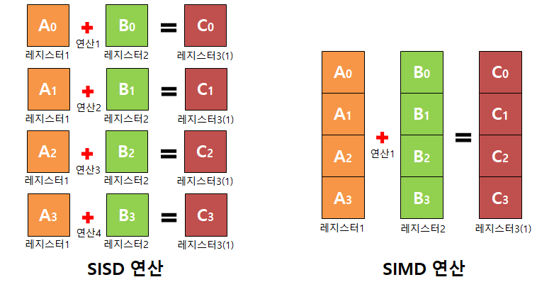
SISDVS SIMD 연산

SIMD: 하나의 명령어로 여러 개의 데이터를 한 번에 처리하는 병렬 방식의 기법의 의미.

Single Instruction Single Data

SISD: 하나의 명령어로 여러 데이터 동시 처리.

Single Instruction Multi Data

때문에 vector, matrix 연산에 적합.

대표적으로 DirectX, OpenGL이 지원.

이를 아래와 같이 코드로 구현해서 비교해보자,
1000000개의 float 정보를 가진 array에 대해 inner product를 진행해보면,
Data Preparation
list_size = 1000000
a = np.random.rand(list_size)
b = np.random.rand(list_size)
loop
def loop() -> float:
	c = 0
	for a_i, b_i in zip(a, b):
		c += a_i * b_i_
	return c
list-comprehension
def listcomp() -> float:
	return sum(a_i + b_i for a_i, b_i in zip(a, b))
vectorized
def vectorized() -> float:
	return np.dot(a, b)
Results
magic command를 사용해서 비교해본 시행 시간은 다음과 같다.
%time func_name()
loop() listcomp() vectorized()
time(ms) 515 549 1.39
원본 링크

	loop()	listcomp()	vectorized()
time(ms)	515	549	1.39

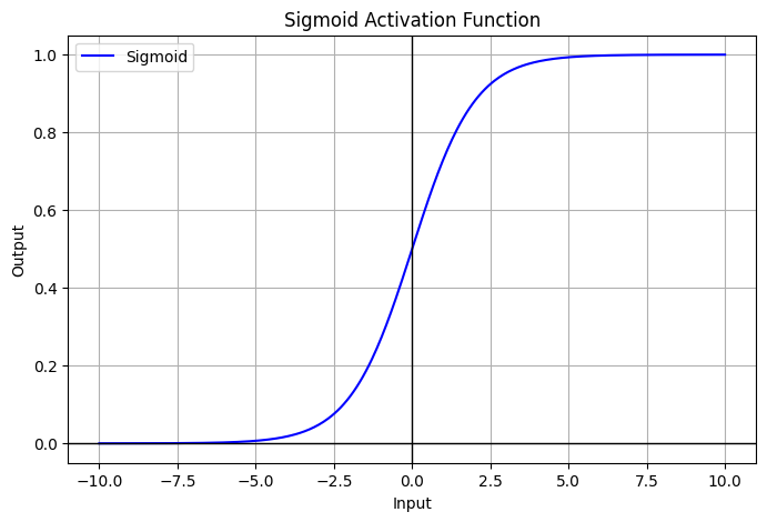
Sigmoid

Sigmoid

activation 중 하나로 대표적으로 많이 사용됨.
$g (x) = \frac{1}{1 + exp ( - x )}$

range: $[0, 1]$

Neuroscience interpretation as saturating “firing rate” of neurons

Problems

Saturation “kills” gradient : 입력 값의 절댓값이 커질수록 기울기 소실

특히나 layer가 깊어질수록, chain-rule에 의해 곱해지는 term들이 많아질텐데, 그러면 앞 쪽에 있는 layer 들일수록 learning되지 않을 수 있지.

Outputs are not zero-centered → introduces bias after the layer

sigmoid와 그 gradient는 항상 positive이기 때문에 model wight의 bias

$y = g (ax + b)$ 라 할 때, $sgn (\partial L / \partial a_{i})$ = $sgn (\partial L / \partial g)$

모든 gradient는 동일한 부호를 가짐.

다음과 같이 구현.
Sigmoid
def sigmoid(x: float) -> float:
	return 1 / (1 + np.exp(-x))
원본 링크

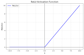
ReLU

ReLU(Rectified Linear Unit)

activation 중 하나로 대표적으로 많이 사용됨.
$g (x) = max (x, 0)$

Does not saturate(for $x > 0$ )

Leads to fast convergence

Computationally efficient

Problems

No learning for $x < 0$ → dead/dying ReLU

downstream gradient가 0(input이 0 이하일 때,)

often initialize with pos. bias ( $b > 0$ )

Outputs are not zero-centered → introduces bias after the layer

sigmoid와 그 gradient는 항상 positive이기 때문에 model wight의 bias

$y = g (ax + b)$ 라 할 때, $sgn (\partial L / \partial a_{i})$ = $sgn (\partial L / \partial g)$

모든 gradient는 동일한 부호를 가짐.

다음과 같이 구현.
ReLU
def relu(x: float) -> float:
	return np.maximum(0, x)
단점들 보안을 위해 Leaky ReLU 등이 있음.

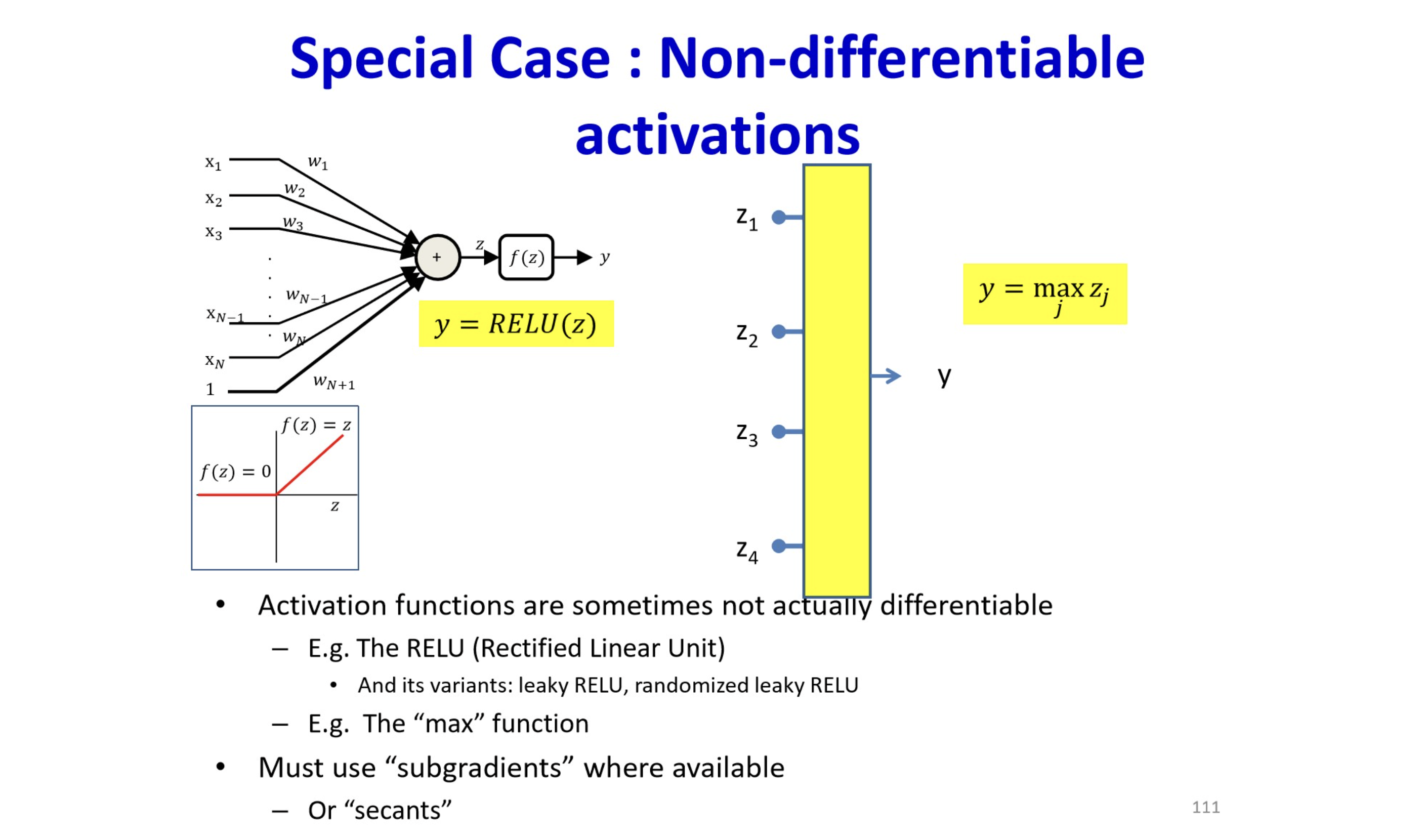
How can we calculate non-differentiable function (like ReLU)?

→ Subgradient

원본 링크

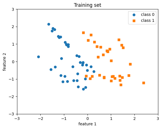
sklearn.datasets

scikit-learn에서 data generation에 용이함.

Sample Code - Generating

import sklearn.datasets as dt
 
data = dt.make_classification(
	n_samples = 100,
	n_features = 2, 
	n_repeated = 0,
	n_classes = 2,
	n_redundant = 0
)
 
X, y = data[0], data[1]
y = y.astype(int)

Sample Code - Shuffling

shuffle_idx = np.arange(y.shape[0])
shuffle_rng = np.random.RandomState(123)
shuffle_rng.shuffle(shuffle_idx)
X, y = X[shuffle_idx], y[shuffle_idx]
 
X_train, X_test = X[shuffle_idx[:70]], X[shuffle_idx[70:]]
y_train, y_test = y[shuffle_idx[:70]], y[shuffle_idx[70:]]

Sample Code - Normalizing

mu, sigma = X_train.mean(axis=0), X_train.std()
X_train = (X_train - mu) / sigma
X_test = (X_test - mu) / sigma

아래 코드로 visualizing하면 다음과 같음.

plot

plt.scatter(X_train[y_train==0, 0], X_train[y_train==0, 1], label='class 0', marker='o')
plt.scatter(X_train[y_train==1, 0], X_train[y_train==1, 1], label='class 1', marker='s')
plt.title('Training set')
plt.xlabel('feature 1')
plt.ylabel('feature 2')
plt.xlim([-3, 3])
plt.ylim([-3, 3])
plt.legend()
plt.show()

원본 링크

Juhyeon's Blog

탐색기

RR04. Perceptrons

MLP(Multi-Layer-Perceptrons)

Vectorization

Sigmoid

ReLU

sklearn.datasets

그래프 뷰

Properties

백링크