MLP(Multi-Layer-Perceptrons)

MLP

Perceptron을 여러 층 쌓은 것.
중간 중간 non-linear function을 사용하여 perceptron을 엮어 더 complex한 function을 approximation 할 수 있음.

Terminology

Net input($z$) = weighted inputs, activation function에 들어갈 값
Activations($a$) = activation function(Net input); $a=\sigma (z)$
Label output($\hat{y}$) = threshold()activations of the last layer; $\hat{y}=f(a)$

Special Cases

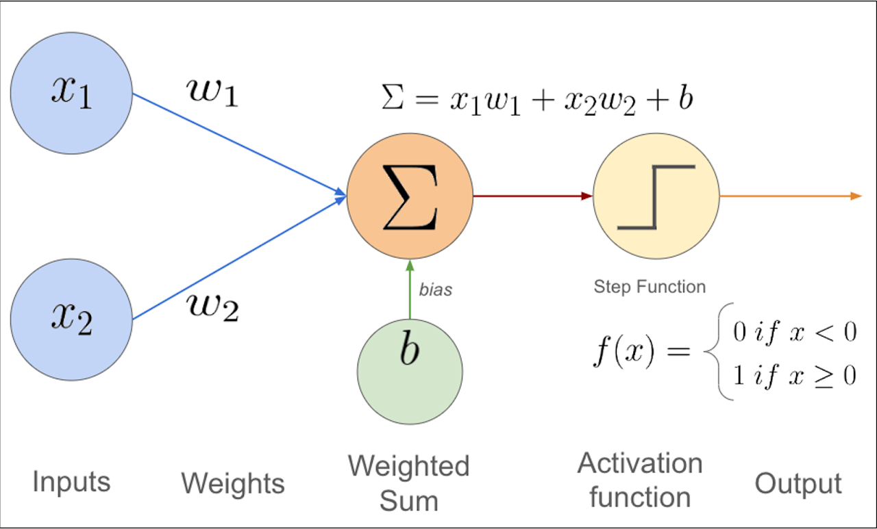
In perceptron: activation function = threshold function(step function)

• 위의 그림에서는 threshold가 0으로 잡혀있음.

In linear regression: activation($a$) = net input($z$) = output($\hat{y}$)

threshold → bias 항으로 몰기

0 & \text{if}\; z \leq \theta \\ 1 & \text{if}\; z > \theta \end{cases}

이를 정리해보면,

0 & \text{if}\; z - \theta \leq 0 \\ 1 & \text{if}\; z - \theta > 0 \end{cases}

여기서 $-\theta$ 를 bias 취급하자.
이를 다시 말하면,
기존
$\sigma ({\sum }_{i=1}^m{x}_i{w}_i+b)=\sigma (x^{T}w+b)=\hat{y}$
input data에서 $x[0]=1$, $w_0=-\theta$ 취급하면 notation이 아래와 같이 간단해진다.
$\sigma ({\sum }_{i=0}^m{x}_i{w}_i)=\sigma (x^{T}w)=\hat{y}$

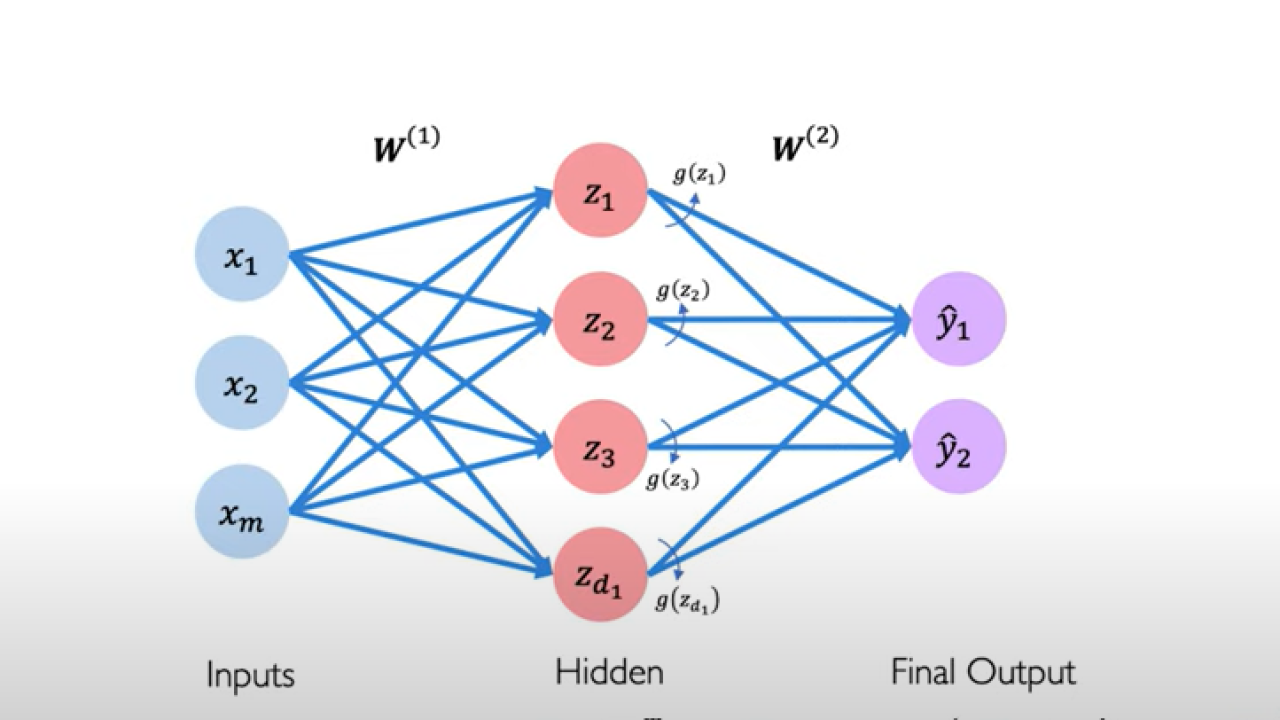
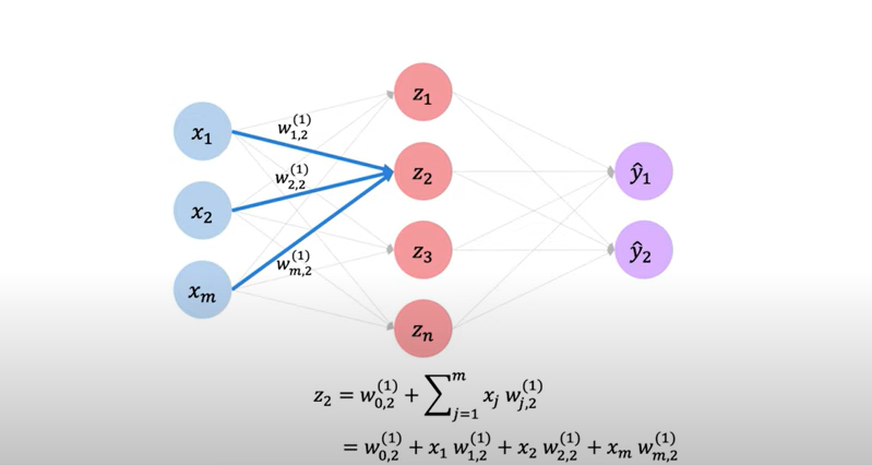
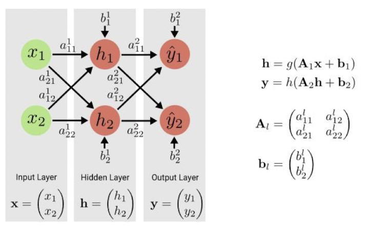
MLP - 1 layer

$z_i=W_{0,i}^{(1)}+{\sum }_{j=1}^m{x}_j{W}_{j,i}^{(1)}$
${\hat{y}}_i=g(W_{0,i}^{(2)}+{\sum }_{j=1}^{d_1}{z}_j{W}_{j,i}^{(2)})$
where $W_{0,i}^{(1)}$, $W_{0,i}^{(2)}$ are bias

앞에 언급한 대로, $W_{0,2}^{(1)}$ 는 bias이므로 input data의 dim을 1 늘리고($x[0]=1$) 로 처리.

Why do we stack more layers?

• 기본적으로 보이는 바와 같이 NN이 깊어질수록 activation을 많이 통과하고 그만큼 non-linearity를 더 부여할 수 있으니 더 complex한 function들을 근사할 수 있지.

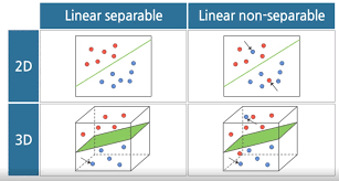
• 또한, 데이터를 linearly separable 하게 바꿀 수도 있지.(e.g. kernel trick 처럼)
  • data를 Linearly-separable 한 space에 embedding 가능.

MLP - 2 layer

Learning MLP

이전에는 manual 하게 파라미터 값들을 define 해주었는데, 이조차도 모델이 스스로 조정하게 하는 걸 학습”Learning” 이라고 함.

• parameter가 많아지면, manual 하게 지정해주는게 intractable
• automatic하게 data로부터 학습하게 할 수 있다는 장점
  → 이러한 접근을 “data-driven approach” or “end-to-end learning” 이라고 함.

Learning Algorithm pseudo-code

Let
$\mathcal{D}=(⟨{\mathbf{x}}^{[1]},y^{[1]}⟩,⟨{\mathbf{x}}^{[2]},y^{[2]}⟩,\cdots ⟨{\mathbf{x}}^{[n]},y^{[n]}⟩)\in ({\mathbb{R}}^m\times \{0,1\}{)}^n$

1. Initialize $\mathbf{w}:=0^m$
2. For every training epochs:
3. For every $⟨{\mathbf{x}}^{[i]},y^{[i]}⟩\in \mathcal{D}$:
   1. ${\hat{y}}^{[i]}:=\sigma ({\mathbf{x}}^{[i]\top }\mathbf{w})$
   2. $\text{err}:=(y^{[i]}-{\hat{y}}^{[i]})$
   3. $\mathbf{w}\leftarrow \mathbf{w}+\text{err}\times {\mathbf{x}}^{[i]}$

2-layer Perceptron

## Modified version of above Perceptron_2layers ##
class Perceptron_2layers():
	def __init__(self, num_features, node):
		self.num_features = num_features
		self.node = node
		self.weights1 = np.zeros((self.num_features, self.node), dtype=float)
		self.weights2 = np.zeros((self.node, 1), dtype=float)
		self.bias1 = np.zeros((1, self.node), dtype=float)
		self.bias2 = np.zeros((1, 1), dtype=float)
		
	def forward(self, x):
		# Forward pass through the network
		# x: (1, num_features) / w1 :(num_features, node) -> z1 : (1, node) -> a1 : (1, node)
		z1 = np.dot(x, self.weights1) + self.bias1 # Linear transformation for hidden layer
		a1 = sigmoid(z1) # Activation for hidden layer
		# a1 : (1, node) / w2 : (node, 1) -> z2 : (1, 1), a2 : (1, 1)
		z2 = np.dot(a1, self.weights2) + self.bias2 # Linear transformation for output layer
		a2 = sigmoid(z2) # Activation for output layer
		predictions = np.where(a2 > 0.5, 1, 0) # Binary predictions
		# z1 : (1, node), a1 : (1, node), z2 : (1, 1), a2 : (1, 1), predictions : (1, 1)
		return z1, a1, z2, a2, predictions
		
	def backward(self, x, y):
		# Backward pass to compute gradients
		# YOUR CODE HERE
		# x:(1, num_features) / y : (1, 1) / predictions : (1, 1)
		z1, a1, z2, a2, predictions = self.forward(x)
		# errors : (1, 1)
		error_output = a2 - y
		# delta_output : (1, 1) / error_hidden : (1, node)
		delta_output = error_output * sigmoid_derivative(z2)
		error_hidden = np.dot(delta_output, self.weights2.T) * sigmoid_derivative(z1)
		return delta_output, error_hidden, a1
		
	def train(self, x, y, epochs, lr=1.):
		for e in range(epochs):
			for i in range(y.shape[0]): # batch_size = 1
			# shaping inputs
				xi = x[i].reshape(1, self.num_features)
				yi = y[i].reshape(1, 1)
				delta_output, error_hidden, a1 = self.backward(xi, yi)
				# Update weights
				self.weights2 -= lr * np.dot(a1.T, delta_output)
				self.bias2 -= lr * delta_output
				self.weights1 -= lr * np.dot(xi.T, error_hidden)
				self.bias1 -= lr * error_hidden
	
	def evaluate(self, x, y):
		# Evaluate the model's performance
		_, _, _, _, predictions = self.forward(x)
		predictions = predictions.reshape(-1)
		accuracy = np.sum(predictions == y) / y.shape[0]
		return accuracy