RR05. Loss Functions

Image Classification

Classification

컴퓨터 비전 분야에서 중요한 task 중 하나로, 이미지 데이터의 label을 예측하는 task.

Challenge - Semantic Gap

---

Semantic Gap

실제 모델이 읽는 값들은 (0, 255) x 3 channel (RGB)범위의 수치들이니, 사람이 이미지 정보 처리 하는 것과는 사뭇 다르다.

• Viewpoint variation : 관측점, 사진이 찍힌 각도에 따라 동일한 대상도 다르게 보인다.
• Illumination: 광량에 따라 대상의 색상 정보 파악이 확연히 다르다.
• Background Clutter: 배경 정보가 경계 구분에 어려움을 줄 수 있다.
• Occlusion : 중요한 정보가 누락될 수 있다.
• Deformation: 같은 객체더라도, 여러 모습이 존재한다.
• Intraclass variation: 같은 클래스 내에도 여러 변산이 존재한다.
• Context: 맥락이 인식에 영향을 준다.

Approach

---

Traditional Approach

---

• 예전에는 feature들을 hard coding하기도 했다고 한다.
• ex) Harris Corner Detection ← 이런 걸 보면 심리학의 “지온” 가설 같은 접근 같기도,,
  • 인접 pixel 간 값 차이가 큰 부분을 detect. → corner ~ boundary

Modern Approach

---

• Data-driven (End-to-End Learning) : DL, ML
  • data 자체로 pattern 인식.
  1. Collect a dataset of images and labels ← big cost,,
     1. CIFAR10, COCO,
  2. Use ML algorithms to train a classifier
  3. Evaluate the classifier on unseen data

원본 링크

Linear Classifiers

Linear classifier

선형 분류기. linearly-separable 한 데이터를 분리할 수 있고, Neural Net은 이 linear-classifier 가 non-linear activation function이랑 묶인 걸로 이해하면 됨.

Parametric Approach : Learning Perceptron(linear classifier)

---

• parameter를 manual하게 researcher가 지정해주는 것이 아닌 흐름.
• Learning은 적절한 parameter를 찾아가는 과정.

• 위의 경우는 CIFAR10을 예시로 사용.
• $x[i]$는 이미지 하나이니, $32\times 32\times 3=3072$ → $\text{x shape:}(3072,1)$
• 분류 타겟 클래스는 총 10개 → $f(x,W)\text{의 shape : }(10,1)$
• → $\text{W의 shape : }(10,3072)$
• if, bias term을 추가한다고 하면, $b\text{의 shape: }(10,1)$

Interpretation

---

• 학습된 weight를 보면, template를 식별한다는 것을 확인할 수 있다.

• geometry 관점에서 보면, 그림과 같이 decision boundary를 기준으로 class 분류를 한다고 해석할 수 있다.
• nn.Linear의 경우, 저걸 column vector로 보면, 출력 dimension 과 같은 개수의 linear classifier로 볼 수 있음.

Limitation

---

• Belows are the challenging scenario that the linear classifiers are hard to classify the data.
  

What(How) to do for finding a good W?

---

• define a objective(Loss Function)
  • how good current classifier
• minimize the loss(Optimization)

원본 링크

CIFAR10

CIFAR-10

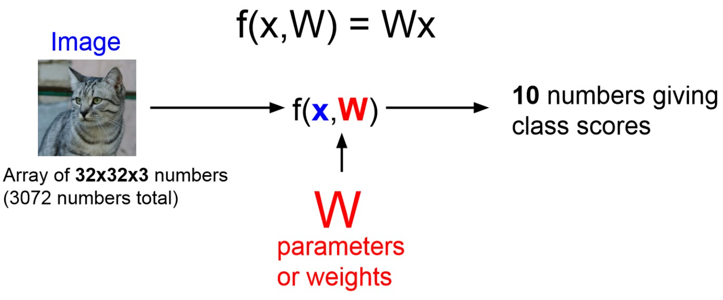
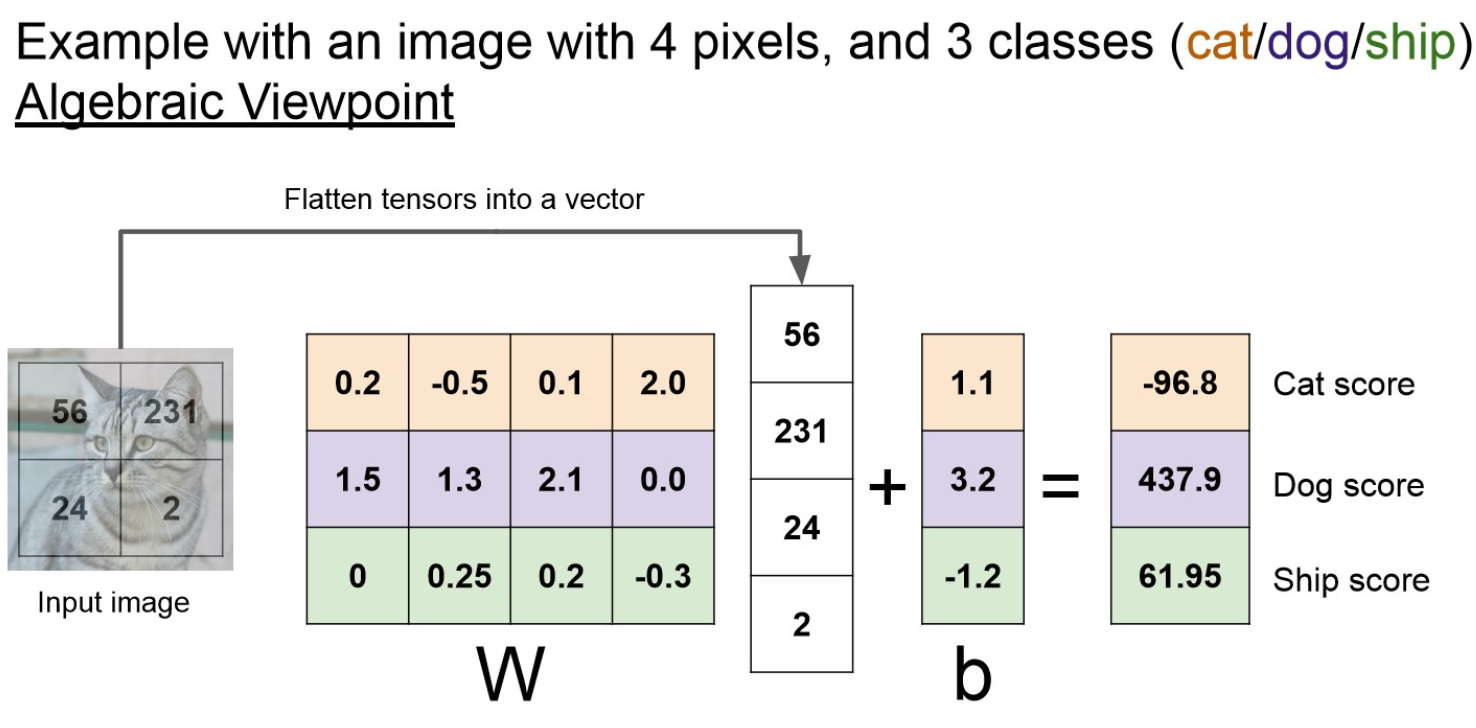
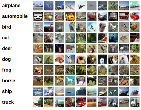
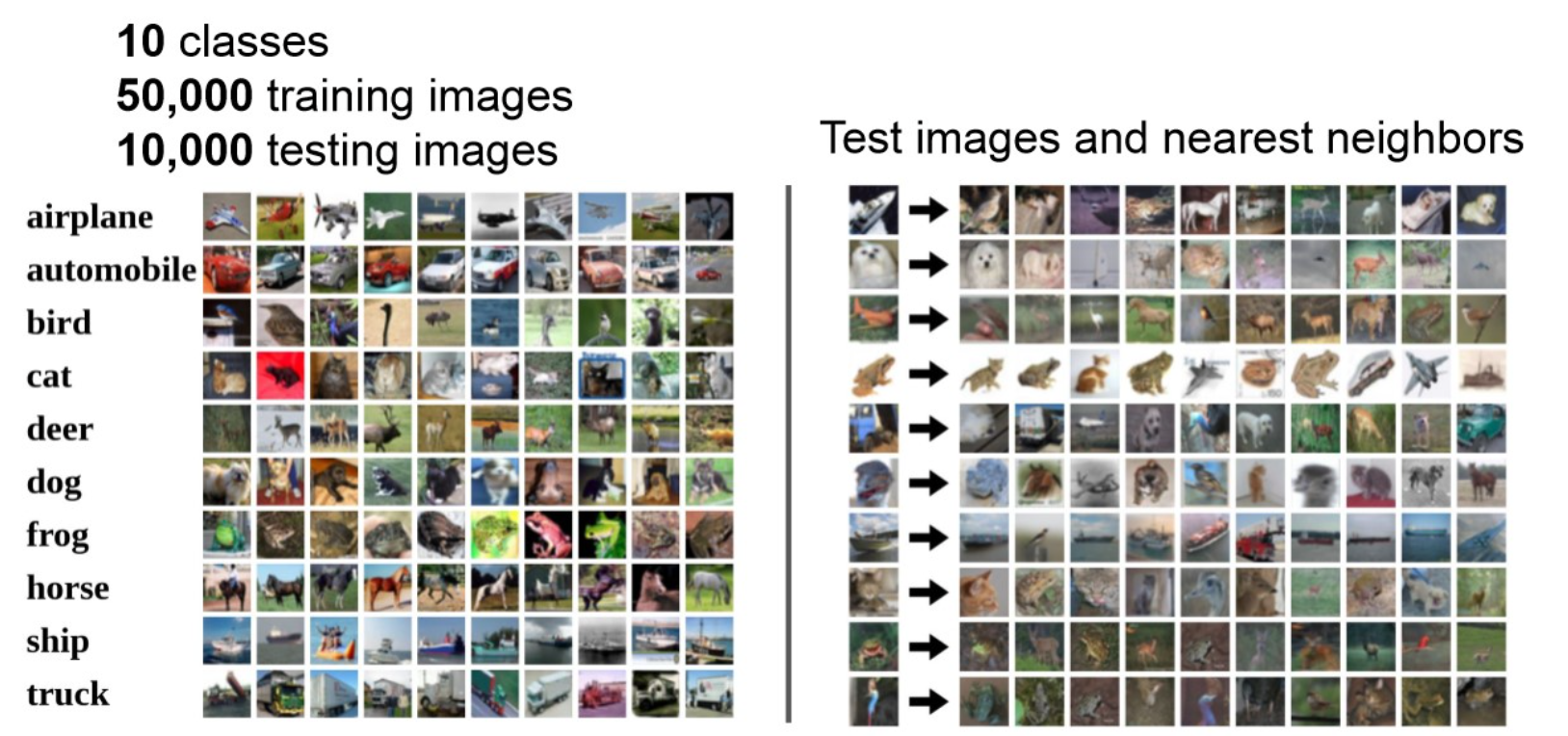
The CIFAR-10 dataset consists of 60000 32x32 colour images in 10 classes, with 6000 images per class. There are 50000 training images and 10000 test images.

원본 링크

Loss Function

Loss(Cost)

Learning 이라는 것은 “Loss”를 “Optimization” 하는 것.
model의 output이랑 target(label)이 최대한 비슷할 때 이 값이 작아지는 방향으로 보통 define함.
확률 분포 간 차이로 볼 수도 있다.

• classification task에서는 마지막 layer가 분류할 target class 개수랑 dim이 같은데, 이를 softmax하면 확률 분포가 model의 최종 output이라고 볼 수 잇다.
• 따라서 learning은 output probability distribution과 target probability distribution을 최대한 비슷하게 해주는 방향으로 진행되어야 한다.
• 확률 분포 차이를 나타내는 지표로 KL-divergence라는 지표를 쓸 수 있고, metric 조건을 정확히 만족하진 못하지만, 대략 distance 개념 정도로 이해할 수 있다.
  • d > 0, d(x, x)=0 → x=0, triangular-ineq

How to design a good loss function?

---

Abstract

• A loss function can be any differentiable function that we wish to optimize
• Deriving the cost function from the Maximum Likelihood Estimation (MLE) principle removes the burden of manually designing the cost function for each model.
• Consider the output of the neural network as parameters of a distribution over $y_i$

${\hat{\mathrm{w}}}_{ML}=\underset{\mathrm{w}}{\mathrm{argmax}}{p}_{model}(\mathrm{y}|\mathrm{X},\mathrm{w})$
$\stackrel{i.i.d}{=}\underset{\mathrm{w}}{\mathrm{argmax}}\prod p_{model}(y_i|X_i,\mathrm{w})$
$=\underset{\mathrm{w}}{\mathrm{argmax}}\sum \text{log}{p}_{model}(y_i|X_i,\mathrm{w})$ (: log-likelihoood 로 변환)

Regression Loss

---

Regression - estimation target

regression이란, 결국
$f_{\mathrm{w}}:{\mathbb{R}}^N\to \mathbb{R}$
즉, output은 real-value 한 개.

• regression을 수행하는 모델이 예측하는 에러 Gaussian distribution으로 보자!
  • target 값은 gaussian의 mean value.

• Mean Square Error(MSE)
• Mean Absolute Error(MAE)
• 여러 분포가 섞인?

Classification Loss

---

Classification - estimation target

classification이란, 결국
$f_{\mathrm{w}}:{\mathbb{R}}^N\to {\mathbb{R}}^N$
즉, output은 real-value vector.

• classification을 수행하는 모델이 예측하는 것은
  • 2 classes: regression with sigmoid로 확률을 바로 뽑던지, 아니면 softmax를 사용.
    • BCE(Binary Cross-Entropy) Loss
  • more than 2: 일반적으로 softmax
    • CE(Cross-Entropy) Loss

• Multiclass SVM Loss
• Binary Cross Entropy
• Cross Entropy

Softmax - Logistic regression

---

Logistic regression

Logistic regression

logistic regression의 경우, linear regression의 output을 확률값 범위로 고정해주는 activation function(tanh)을 적용한 걸로 볼 수도 있는데, classification task에 수행할 수 있다는 점을 잘 기억하자!
→ ouput 값이 확률 값의 범위에 무조건 떨어지니까.
수식으로는 아래와 같이 model 을 define하고,
$h(\mathrm{x})=\sigma ({\mathrm{w}}^{\top }\mathrm{x}+b)$
model의 output을 posterior 해석.

h(\mathrm{x}) & \text{if}\; y = 1 \\ 1 - h(\mathrm{x}) & \text{if}\; y = 0 \end{cases}$$ 이걸 좀 compact 하게 한 줄로 써보면, $$P(y|\mathrm{x}) = a^y(1-a)^{(1-y)}$$

원본 링크

Expand to BCE

위의 식에서 여러 개의 데이터가 i.i.d. 가정을 통해 뽑혔다고 한다면,
$P(y^{[1]},\cdots ,y^{[n]}|{\mathrm{x}}^{[1]},\cdots ,{\mathrm{x}}^{[n]})=\prod P(y^{[i]}|{\mathrm{x}}^{[i]})$
여기서, MLE
$L(\mathrm{w})=P(\mathrm{y}|\mathrm{x};\mathrm{w})$
$=\prod P(y^{[i]}|x^{[i]};\mathrm{w})$
$\prod (\sigma (z^{[i]}){)}^{y^{[i]}}(1-\sigma (z^{[i]}){)}^{(1-y^{[i]})}$
where $z^{[i]}={\mathrm{w}}^{\top }\mathrm{x}+b$
실제 compute 할 때에는 log 씌우는 게 값이 stable하여 log를 씌운 이후 계산한다고 하는데 정확히 어떠한 말일까..?

$l(\mathrm{w})=\text{log}L(\mathrm{w})$
$=\sum [y^{[i]}\text{log}(\sigma (z^{[i]}))+(1-y^{[i]})\text{log}(1-\sigma (z^{[i]}))]$
또한, 값을 maximizing 하는 것 보다는 minimizing 하는게 편하기 때문에(??) negative log-likelihood를 minimizing 한다.
$L(\mathrm{w})=-l(\mathrm{w})$
$=-\sum [y^{[i]}\text{log}(\sigma (z^{[i]}))+(1-y^{[i]})\text{log}(1-\sigma (z^{[i]}))]$

Expand to Multiple Classes

Categorical distribution을 다음과 같이 정의
$p(y=c)={\mu }_c$
따라서 probability distribution은
$p(\mathrm{y})=\prod {\mu }_c^{y_c}$
로 표현될 수 있고,
$\mathrm{y}$: One-hot vector로 $y_c\in \{0,1\}$

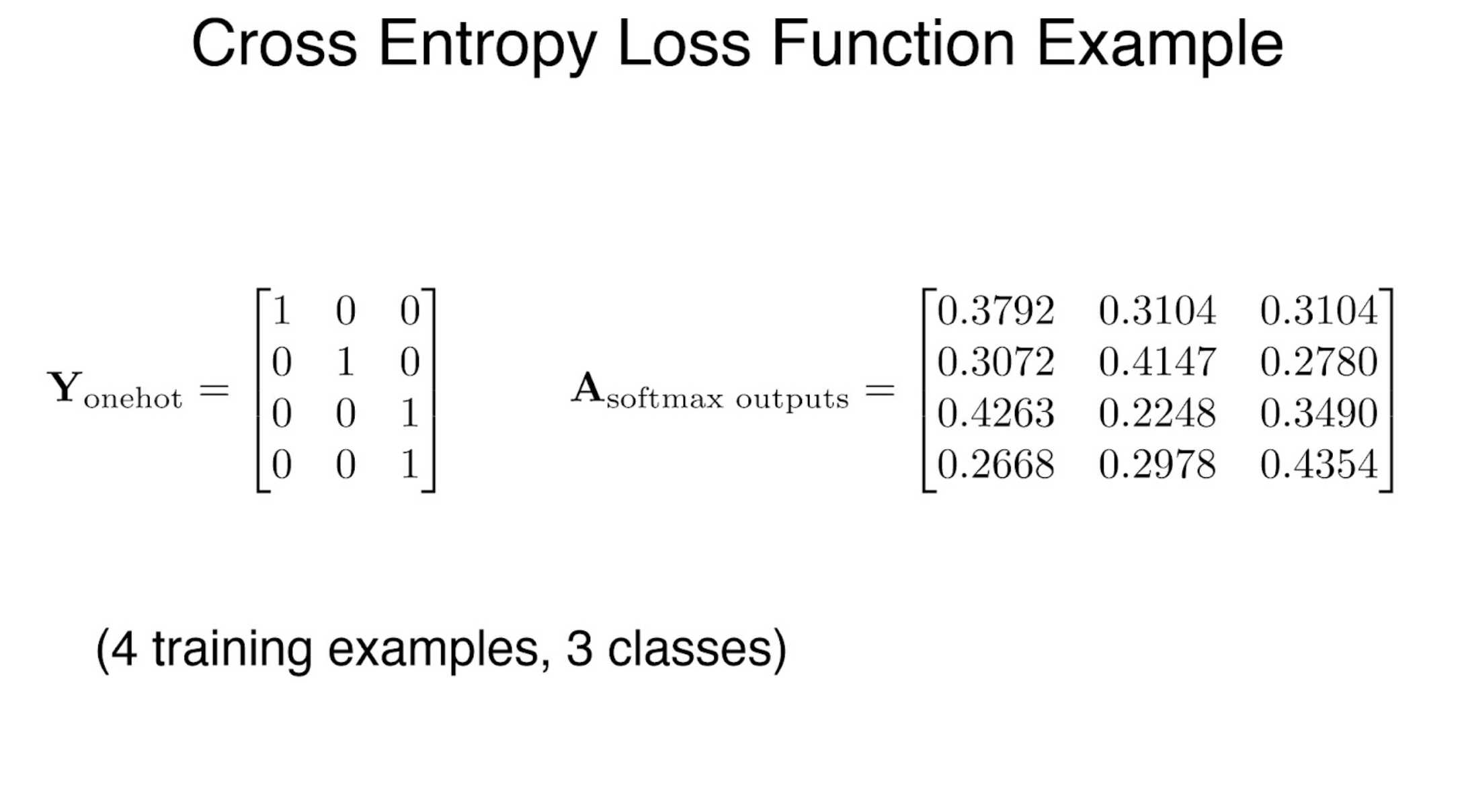
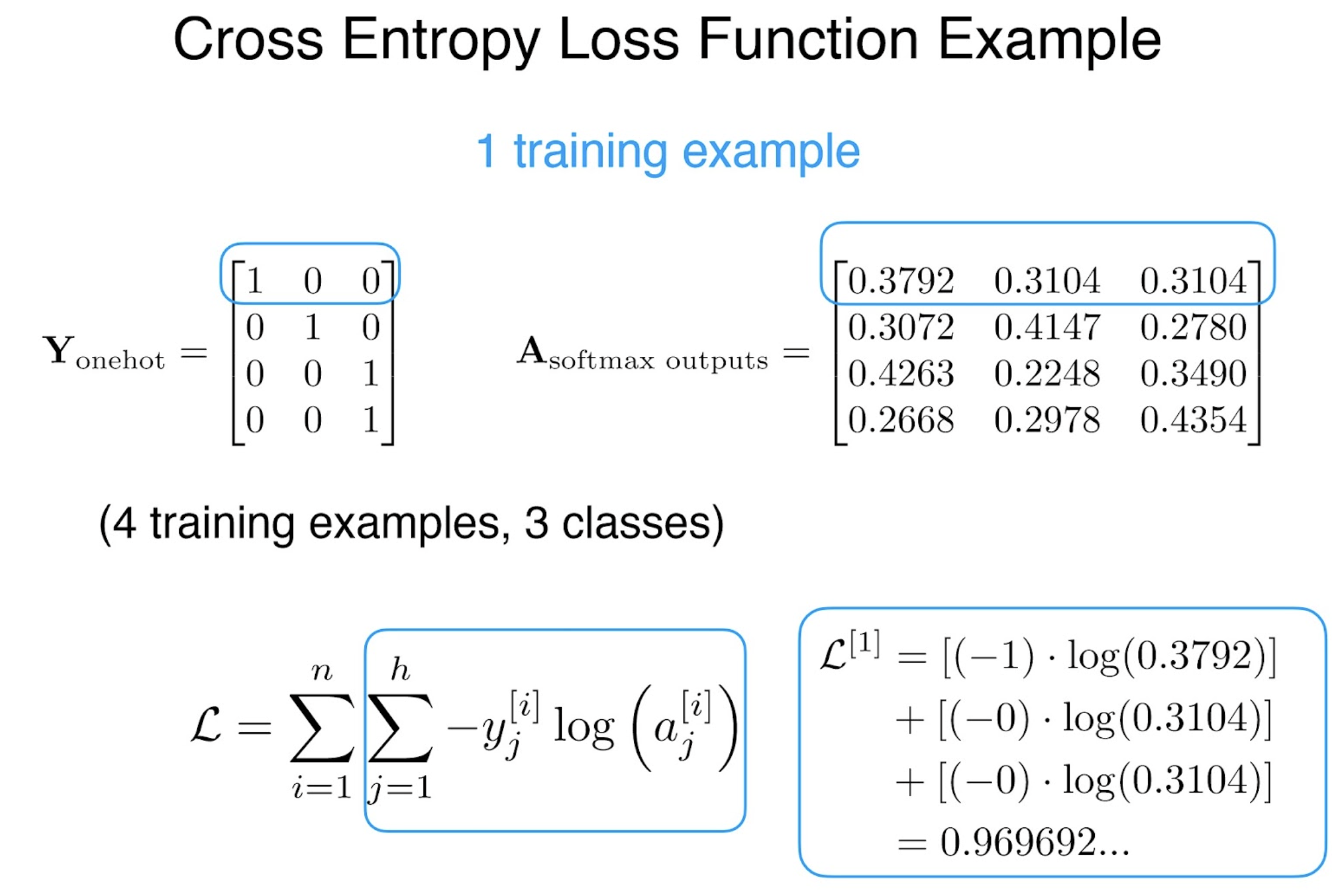
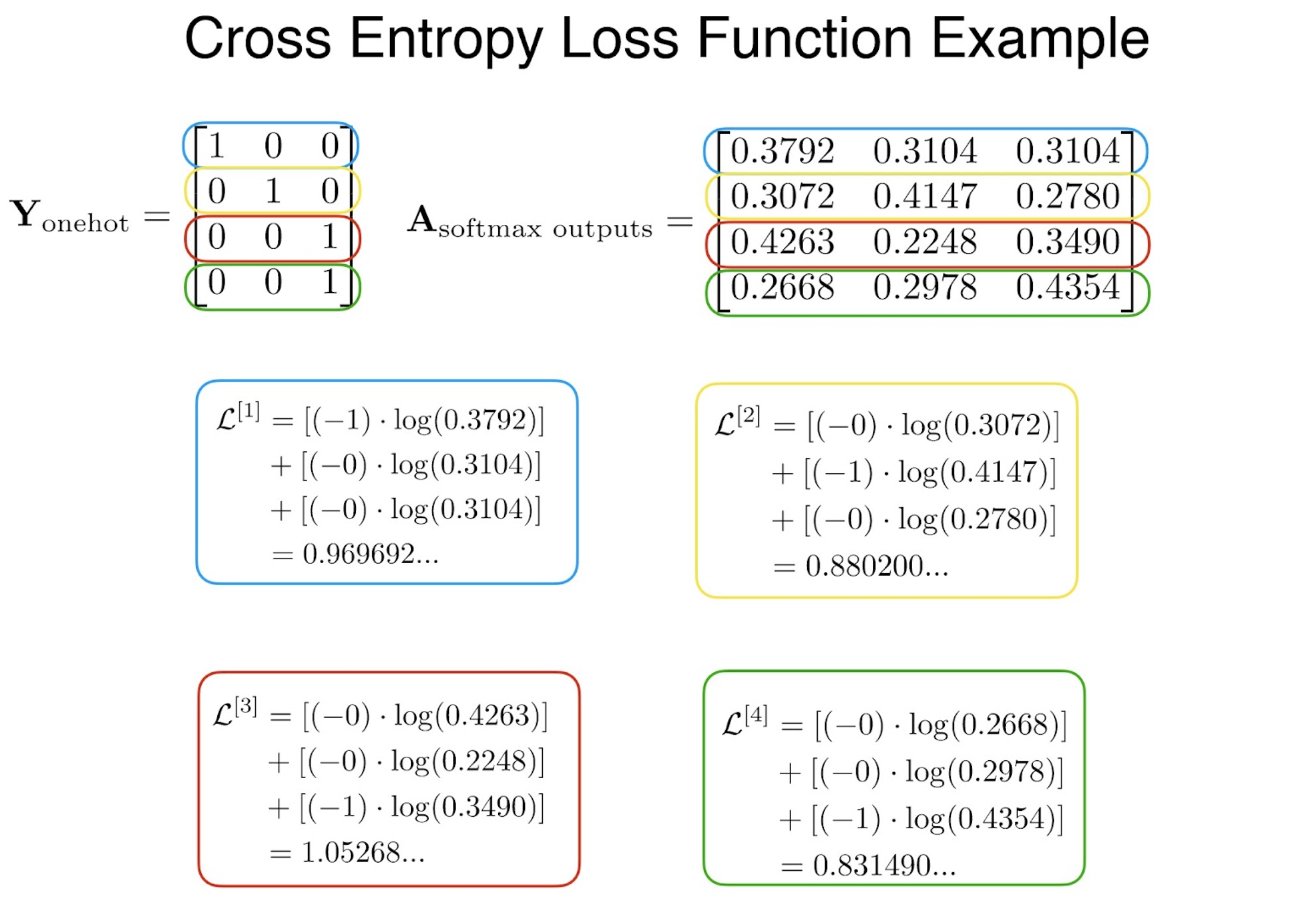
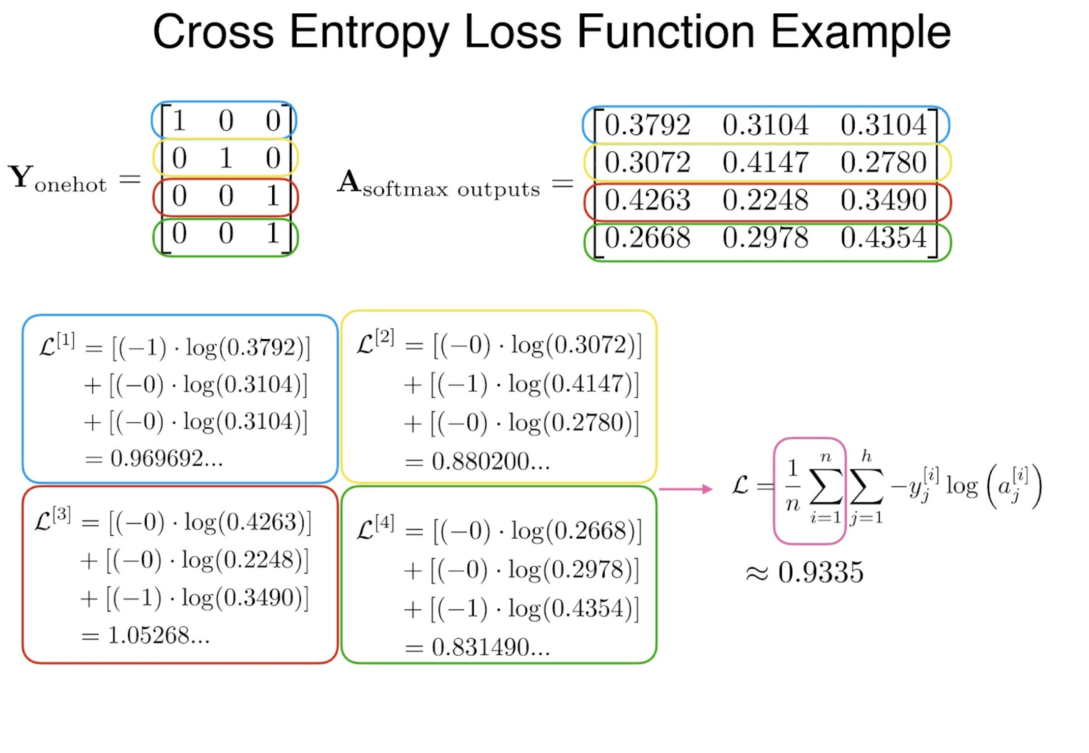
CE(Cross-Entropy) Loss?

Let $P_{model}(\mathrm{y}|\mathrm{x},\mathrm{w})=\prod f_{\mathrm{w}}^{(c)}(\mathrm{x}{)}^{y_c}$
then we obtain,
${\hat{\mathrm{w}}}_{ML}=\underset{\mathrm{w}}{\mathrm{argmax}}\sum \text{log}{p}_{model}(y_i|x_i,\mathrm{w})$

$=\underset{\mathrm{w}}{\mathrm{argmax}}\sum \text{log}\prod f_{\mathrm{w}}^{(c)}(\mathrm{x}{)}^{y_c}$

$=\underset{\mathrm{w}}{\mathrm{argmin}}{\sum }_{i=1}^N{\sum }_{c=1}^C-y_{i,c}\text{log}{f}_{\mathrm{w}}^{(c)}({\mathrm{x}}_i)$

In other words, we minimize the cross-entropy loss(CE loss).
The target $\mathrm{y}=(0,0,\cdots ,0,\cdots ,0{)}^{\top }$ is a One-hot vector with $y_c$ its c’th element.

CE-Loss

원본 링크

Recitation

---

Perceptron

Perceptron

input들의 weighted sum된 값에 threshold(step-function)을 적용해서 binary 값을 return

Consider a simple model
$\hat{y}=f(x;w,b)=w_1{x}_1+w_2{x}_2+b$
can be represent as a $\hat{y}=w^{\mathrm{T}}x+b$ where $w=[w_1,w_2]$ and $x=[x_1,x_2]$ .

이렇게 linear model에서 weighted sum을 계산한 뒤에 threshold값 기준으로 이상인지, 미만인지 판단하여 binary를 return.

Logical AND Gate

---

Logical AND

Summary

아래와 같은 gate를 만들고 싶은 것.

$x_1$	$x_2$	$Out$
0	0	0
0	1	0
1	0	0
1	1	1
이를 모형화 하면,
이렇게 되는데, threshold는 W에 depend.

원본 링크

Logical OR Gate

---

Logical OR

Summary

아래와 같은 gate를 만들고 싶은 것.

$x_1$	$x_2$	$Out$
0	0	0
0	1	1
1	0	1
1	1	1
이를 모형화 하면,
이렇게 되는데, threshold는 W에 depend.

원본 링크

마찬가지로, logical NAND에 대해서도 가능.
NAND = NOT(AND)

XOR problem

---

XOR problem

• Visually, not linearly separable 해보이는데..?
• Convex 개념 가져와서 보면,

NOTE

Half spaces(e.g., decision regieon) are convex set.
즉, linear classifier가 나누는 두 영역도 convex set.

NOTE

Suppose there was a feasible hypothesis. If the positive examples are in the positive half-space, then the green line segment must as well.

원본 링크

Convex

---

Convex

Summary

함수가 아래로 볼록하냐? : convex
위로 볼록(=아래로 오목) : concave

Definition

---

A set $\mathcal{S}$ is convex if any line segment connecting 2 points in $\mathcal{S}$ lies entirely within $\mathcal{S}$.
$x_1,x_2\in S⟹\lambda x_1+(1-\lambda )x_2\in S$for $\lambda \in [0,1]$ .

In the perspective of Optimization…

---

NOTE

Optimization 관점에서 봤을 때, 함수가 convex 하다면, global minima가 한 개라는 말이니까, GD의 destination이 무조건 global minima 겠지.

원본 링크

MLP

—

이름 그대로 위의 perceptron을 multi-layer 쌓아서 적층한 구조. 각 layer에서 다음 layer로 넘어가는 과정에서 non-linear function을 통과하니, 이때 점차 model에 non-linearity가 생김. 따라서 이러한 구조가 3층이상으로 깊게 쌓이면 Deep-Neural-Network이라 함. 

SIMD(Single Instruction Multiple Data)

—

여러 개의 data를 vector 형식으로 묶어서 처리하자!

**

파이썬으로 구현해보기!

Perceptron

class Perceptron():
	def __init__(self, num_features):
		self.num_features = num_features
		self.weights = np.zeros((num_features, 1), dtype=float)
		self.bias = np.zeros(1, dtype=float)
	
	def forward(self, x):
		# $\hat{y} = xw + b$
		linear = np.dot(x, self.weights) + self.bias # comp. net input
		# train에서 보면, y[i] 차원으로 데이터가 들어오니, vec * vec 연산.
		# linear = x @ self.weights + self.bias
		predictions = np.where(linear > 0., 1, 0) # step function - threshold
		return predictions
		
	# 'ppp' exercise
	def backward(self, x, y):
		# pred랑 ground_truth 값 비교.
		return y - self.forward(x)
		
	# 중간 중간 reshape이 과연 필요할까?
	def train(self, x, y, epochs):
		for e in range(epochs):
			for i in range(y.shape[0]):
				errors = self.backward(x[i].reshape(1, self.num_features), y[i]).reshape(-1)
				self.weights += (errors * x[i]).reshape(self.num_features, 1)
				self.bias += errors
	def evaluate(self, x, y):
		predictions = self.forward(x).reshape(-1)
		accuracy = np.sum(predictions == y) / y.shape[0]
		return accuracy

Perceptron-Vectorized version

class Perceptron_vec():
	def __init__(self, num_features):
		self.num_features = num_features
		self.weights = np.zeros((num_features, 1), dtype=float)
		self.bias = np.zeros(1, dtype=float)
		
	def forward(self, x):
		# x: (n, n_features) / weights: (num_features, 1) -> np.dot(x, self.weights) : (n, 1)
		# therefore, self.bias will be broadcasted. self.bias : (1, ) -> (n, )
		# linear : (n, 1) + (n, ) -> (n, 1)
		linear = np.dot(x, self.weights) + self.bias
		# predictions: (n, 1)
		predictions = np.where(linear > 0.5, 1, 0)
		return predictions
		
	def backward(self, x, y):
		# predictions : (n, 1)
		predictions = self.forward(x)
		# errors: (n, 1)
		errors = y - predictions
		return errors
		
	# 'ppp' exercise
	# YOUR CODE HERE
	def train(self, x, y, epochs):
		for e in range(epochs):
			# errors: (n, 1)
			errors = self.backward(x, y.reshape(y.shape[0], 1))
			# self.weights: (n_features, 1)
			# x.T : (n_features, n) / errors: (n, 1)
			self.weights+= np.dot(x.T, errors) # parameter update
			self.bias += errors.mean()
			
	def evaluate(self, x, y):
		predictions = self.forward(x).reshape(-1)
		accuracy = np.sum(predictions == y) / y.shape[0]
		return accuracy

Training Code

ppn = Perceptron(num_features = 2)
 
pp.train(X_train, y_train, epochs=5)
 
print('Model parameters:\n\n')
print('Weights: %s\n ' % ppn.weights)
print('Bias: %s\n ' % ppn.bias)

Evaluating Code

train_acc = ppn.evaluate(X_train, y_train)
print('Train set accuracy: %.2f ' % (test_acc*100))

Decision Boundary plot

##########################
### 2D Decision Boundary
##########################
w, b = ppn.weights, ppn.bias
 
x0_min = -2
x1_min = ((-(w[0] * x0_min) - b[0]) / w[1])
 
x0_max = 2
x1_max = ((-(w[0] * x0_max) - b[0]) / w[1])
 
# x0*w0 + x1*w1 + b = 0
# x1 = (-x0*w0 - b) / w1
# 'ppp' exercise
 
import matplotlib.pyplot as plt
fig, ax = plt.subplots(nrows=1, ncols=2, sharex = True, figsize=(10, 5))
 
for idx, ax_i in enumerate(ax):
	ax_i.plot([x0_min, x0_max], [x1_min, x1_max]) # decision boundary
	ax_i.set_xlabel('feature 1')
	ax_i.set_ylabel('feature 2')
	ax_i.set_xlim([-3, 3])
	ax_i.set_ylim([-3, 3])
	
	if idx == 0:
		ax_i.set_title('Training set')
		ax_i.scatter(X_train[y_train==0, 0], X_train[y_train==0, 1], label='class 0', marker='o')
		ax_i.scatter(X_train[y_train==1, 0], X_train[y_train==1, 1], label='class 1', marker='s')
	else:
		ax_i.set_title('Test set')
		ax_i.scatter(X_test[y_test==0, 0], X_test[y_test==0, 1], label='class 0', marker='o')
		ax_i.scatter(X_test[y_test==1, 0], X_test[y_test==1, 1], label='class 1', marker='s')
		
	ax_i.legend(loc='upper left')
	plt.show()

원본 링크

MLP(Multi-Layer-Perceptrons)

MLP

Perceptron을 여러 층 쌓은 것.
중간 중간 non-linear function을 사용하여 perceptron을 엮어 더 complex한 function을 approximation 할 수 있음.

Terminology

Net input($z$) = weighted inputs, activation function에 들어갈 값
Activations($a$) = activation function(Net input); $a=\sigma (z)$
Label output($\hat{y}$) = threshold()activations of the last layer; $\hat{y}=f(a)$

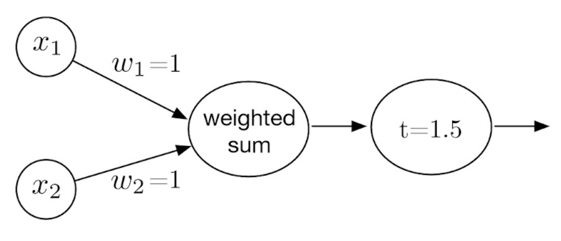
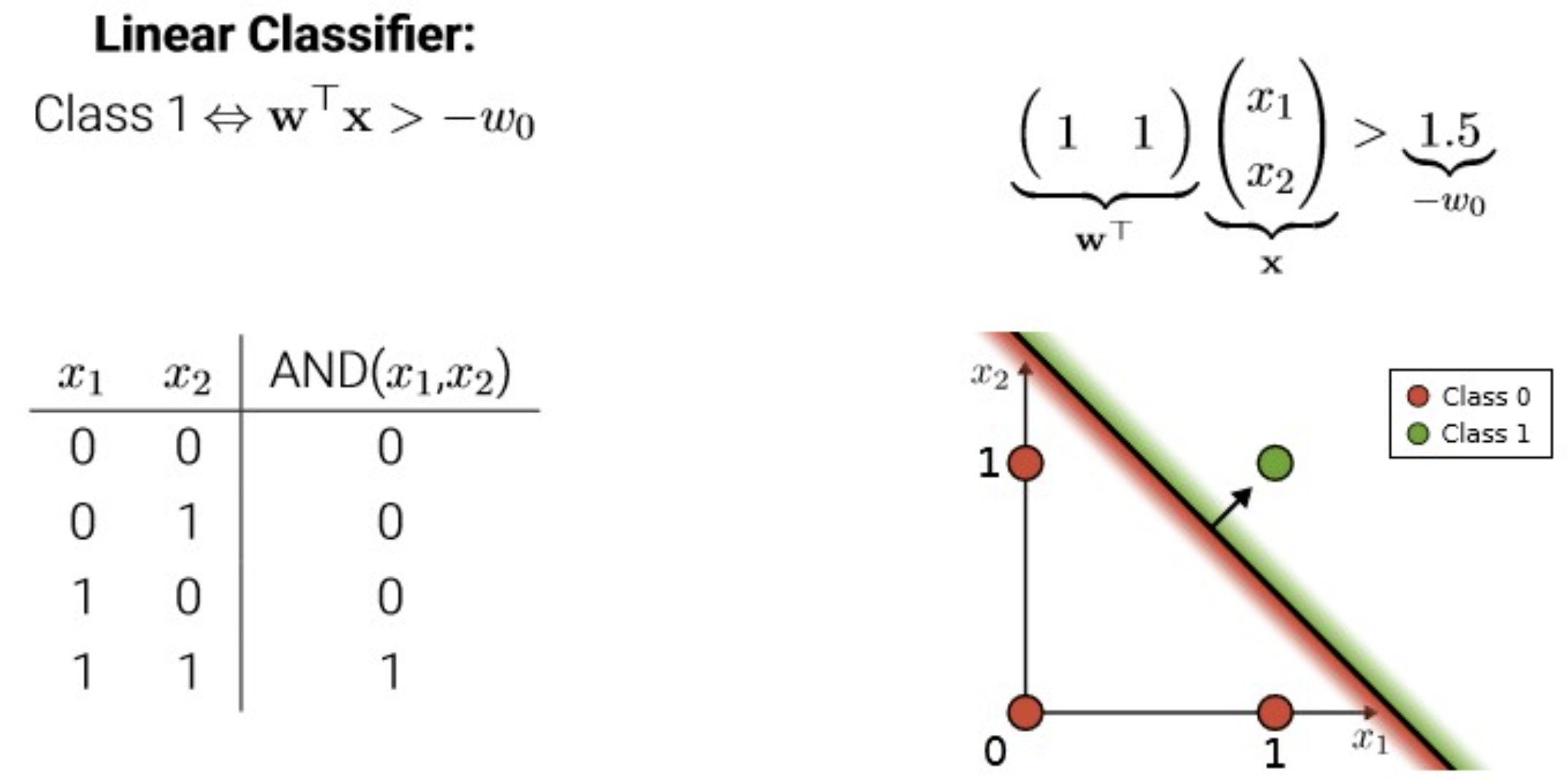
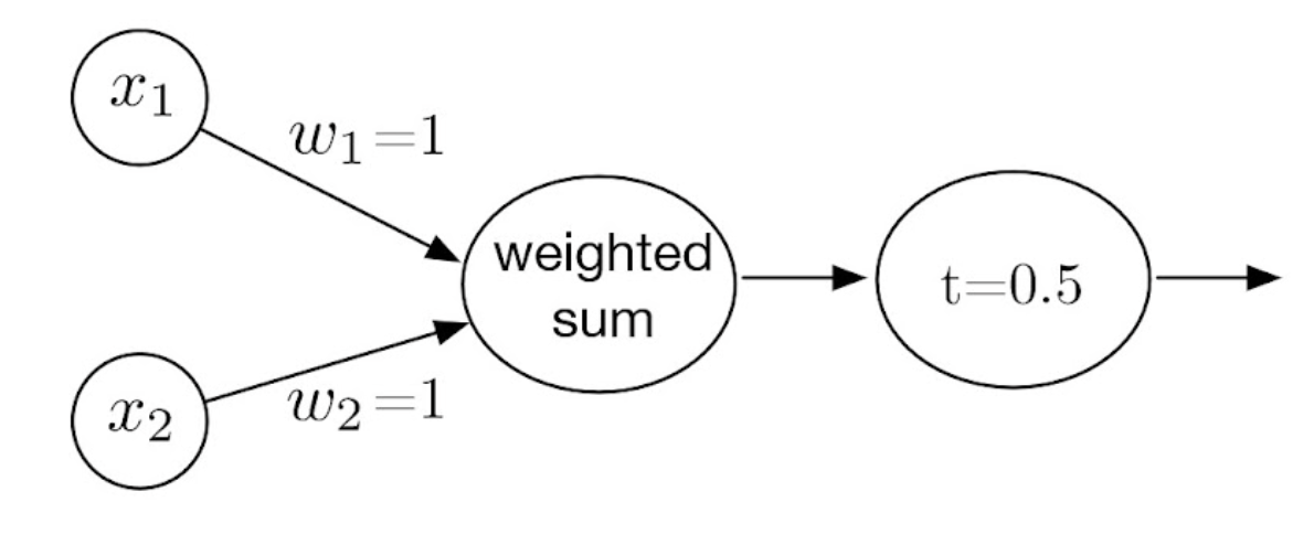
Special Cases

In perceptron: activation function = threshold function(step function)

• 위의 그림에서는 threshold가 0으로 잡혀있음.

In linear regression: activation($a$) = net input($z$) = output($\hat{y}$)

threshold → bias 항으로 몰기

0 & \text{if}\; z \leq \theta \\ 1 & \text{if}\; z > \theta \end{cases}

이를 정리해보면,

0 & \text{if}\; z - \theta \leq 0 \\ 1 & \text{if}\; z - \theta > 0 \end{cases}

여기서 $-\theta$ 를 bias 취급하자.
이를 다시 말하면,
기존
$\sigma ({\sum }_{i=1}^m{x}_i{w}_i+b)=\sigma (x^{T}w+b)=\hat{y}$
input data에서 $x[0]=1$, $w_0=-\theta$ 취급하면 notation이 아래와 같이 간단해진다.
$\sigma ({\sum }_{i=0}^m{x}_i{w}_i)=\sigma (x^{T}w)=\hat{y}$

MLP - 1 layer

$z_i=W_{0,i}^{(1)}+{\sum }_{j=1}^m{x}_j{W}_{j,i}^{(1)}$
${\hat{y}}_i=g(W_{0,i}^{(2)}+{\sum }_{j=1}^{d_1}{z}_j{W}_{j,i}^{(2)})$
where $W_{0,i}^{(1)}$, $W_{0,i}^{(2)}$ are bias

앞에 언급한 대로, $W_{0,2}^{(1)}$ 는 bias이므로 input data의 dim을 1 늘리고($x[0]=1$) 로 처리.

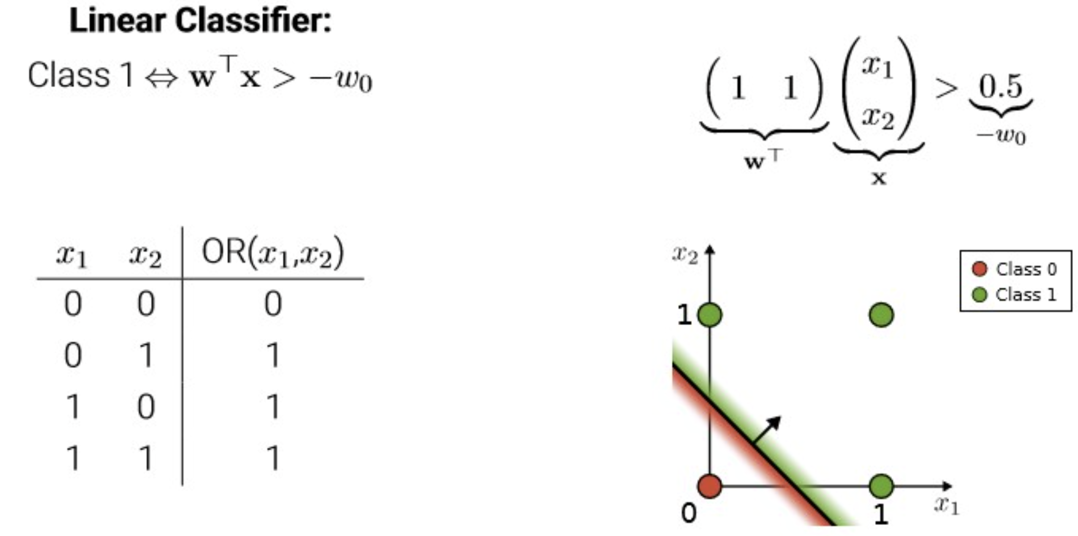
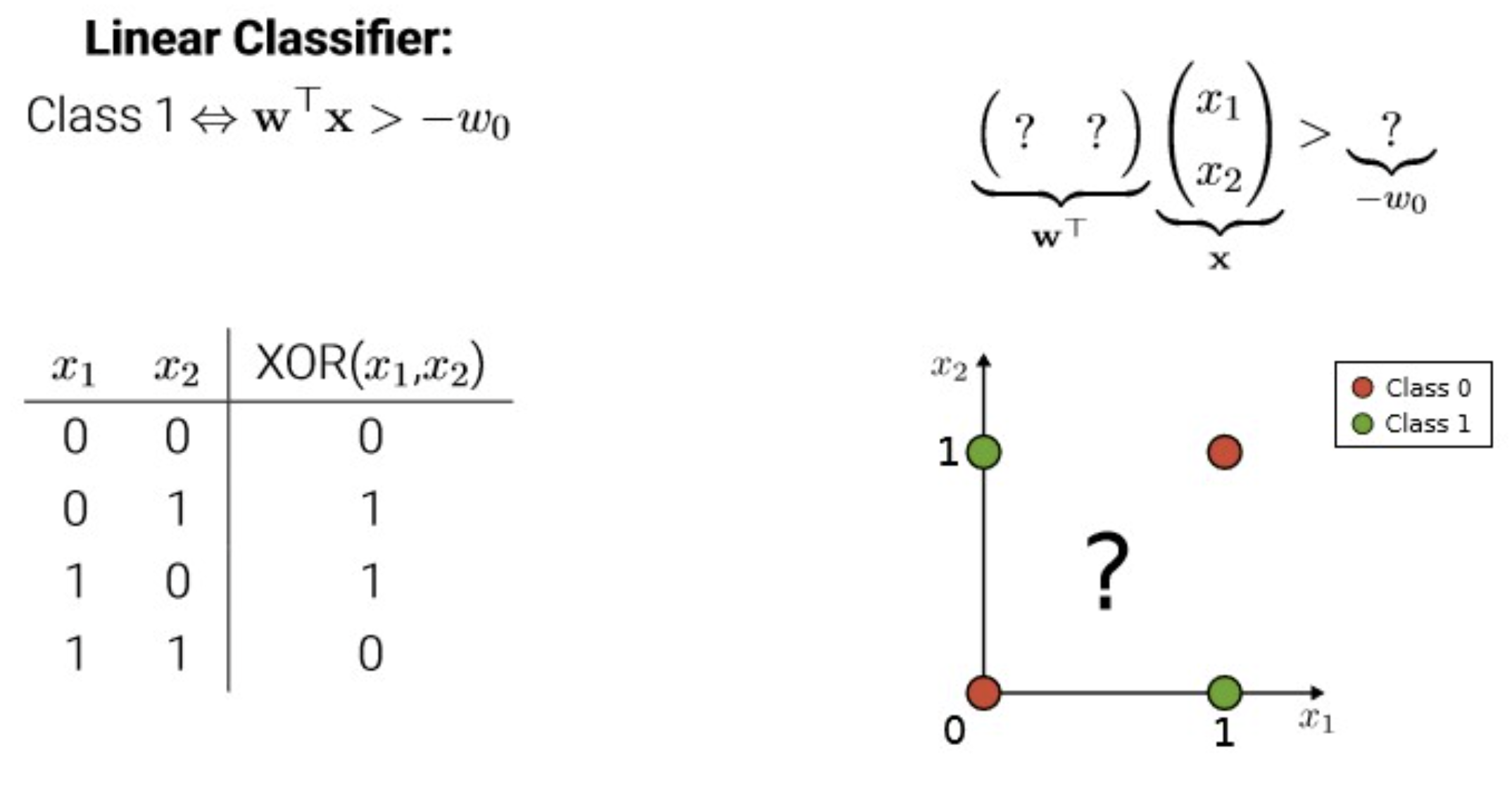
Why do we stack more layers?

• 기본적으로 보이는 바와 같이 NN이 깊어질수록 activation을 많이 통과하고 그만큼 non-linearity를 더 부여할 수 있으니 더 complex한 function들을 근사할 수 있지.

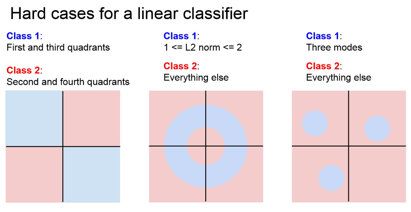
• 또한, 데이터를 linearly separable 하게 바꿀 수도 있지.(e.g. kernel trick 처럼)
  • data를 Linearly-separable 한 space에 embedding 가능.

MLP - 2 layer

Learning MLP

이전에는 manual 하게 파라미터 값들을 define 해주었는데, 이조차도 모델이 스스로 조정하게 하는 걸 학습”Learning” 이라고 함.

• parameter가 많아지면, manual 하게 지정해주는게 intractable
• automatic하게 data로부터 학습하게 할 수 있다는 장점
  → 이러한 접근을 “data-driven approach” or “end-to-end learning” 이라고 함.

Learning Algorithm pseudo-code

Let
$\mathcal{D}=(⟨{\mathbf{x}}^{[1]},y^{[1]}⟩,⟨{\mathbf{x}}^{[2]},y^{[2]}⟩,\cdots ⟨{\mathbf{x}}^{[n]},y^{[n]}⟩)\in ({\mathbb{R}}^m\times \{0,1\}{)}^n$

1. Initialize $\mathbf{w}:=0^m$
2. For every training epochs:
3. For every $⟨{\mathbf{x}}^{[i]},y^{[i]}⟩\in \mathcal{D}$:
   1. ${\hat{y}}^{[i]}:=\sigma ({\mathbf{x}}^{[i]\top }\mathbf{w})$
   2. $\text{err}:=(y^{[i]}-{\hat{y}}^{[i]})$
   3. $\mathbf{w}\leftarrow \mathbf{w}+\text{err}\times {\mathbf{x}}^{[i]}$

2-layer Perceptron

## Modified version of above Perceptron_2layers ##
class Perceptron_2layers():
	def __init__(self, num_features, node):
		self.num_features = num_features
		self.node = node
		self.weights1 = np.zeros((self.num_features, self.node), dtype=float)
		self.weights2 = np.zeros((self.node, 1), dtype=float)
		self.bias1 = np.zeros((1, self.node), dtype=float)
		self.bias2 = np.zeros((1, 1), dtype=float)
		
	def forward(self, x):
		# Forward pass through the network
		# x: (1, num_features) / w1 :(num_features, node) -> z1 : (1, node) -> a1 : (1, node)
		z1 = np.dot(x, self.weights1) + self.bias1 # Linear transformation for hidden layer
		a1 = sigmoid(z1) # Activation for hidden layer
		# a1 : (1, node) / w2 : (node, 1) -> z2 : (1, 1), a2 : (1, 1)
		z2 = np.dot(a1, self.weights2) + self.bias2 # Linear transformation for output layer
		a2 = sigmoid(z2) # Activation for output layer
		predictions = np.where(a2 > 0.5, 1, 0) # Binary predictions
		# z1 : (1, node), a1 : (1, node), z2 : (1, 1), a2 : (1, 1), predictions : (1, 1)
		return z1, a1, z2, a2, predictions
		
	def backward(self, x, y):
		# Backward pass to compute gradients
		# YOUR CODE HERE
		# x:(1, num_features) / y : (1, 1) / predictions : (1, 1)
		z1, a1, z2, a2, predictions = self.forward(x)
		# errors : (1, 1)
		error_output = a2 - y
		# delta_output : (1, 1) / error_hidden : (1, node)
		delta_output = error_output * sigmoid_derivative(z2)
		error_hidden = np.dot(delta_output, self.weights2.T) * sigmoid_derivative(z1)
		return delta_output, error_hidden, a1
		
	def train(self, x, y, epochs, lr=1.):
		for e in range(epochs):
			for i in range(y.shape[0]): # batch_size = 1
			# shaping inputs
				xi = x[i].reshape(1, self.num_features)
				yi = y[i].reshape(1, 1)
				delta_output, error_hidden, a1 = self.backward(xi, yi)
				# Update weights
				self.weights2 -= lr * np.dot(a1.T, delta_output)
				self.bias2 -= lr * delta_output
				self.weights1 -= lr * np.dot(xi.T, error_hidden)
				self.bias1 -= lr * error_hidden
	
	def evaluate(self, x, y):
		# Evaluate the model's performance
		_, _, _, _, predictions = self.forward(x)
		predictions = predictions.reshape(-1)
		accuracy = np.sum(predictions == y) / y.shape[0]
		return accuracy

원본 링크