RR02. Preliminaries -2

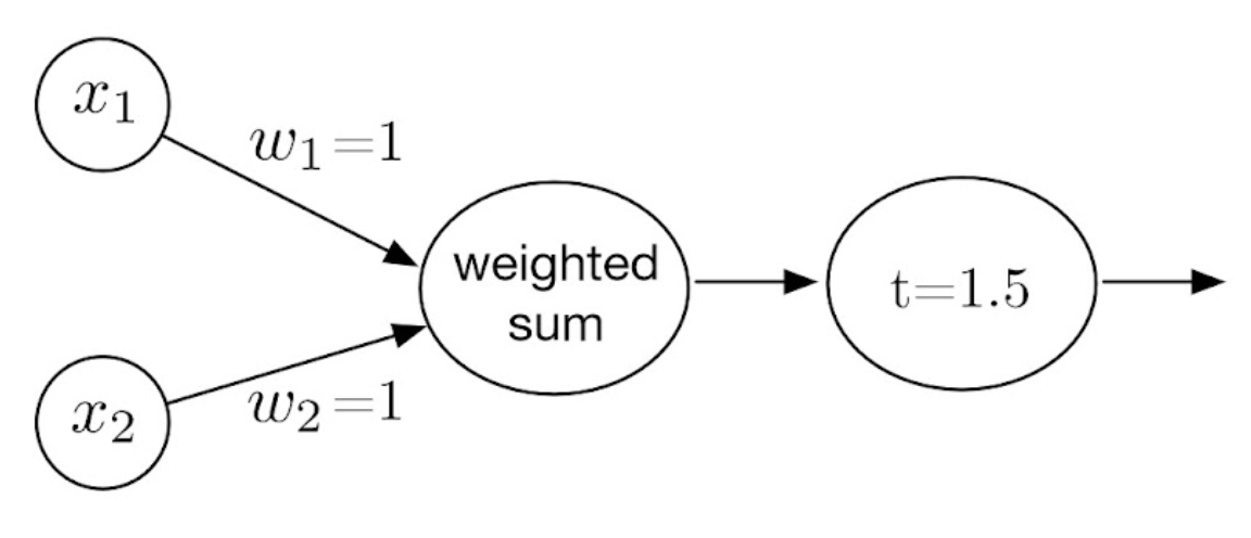
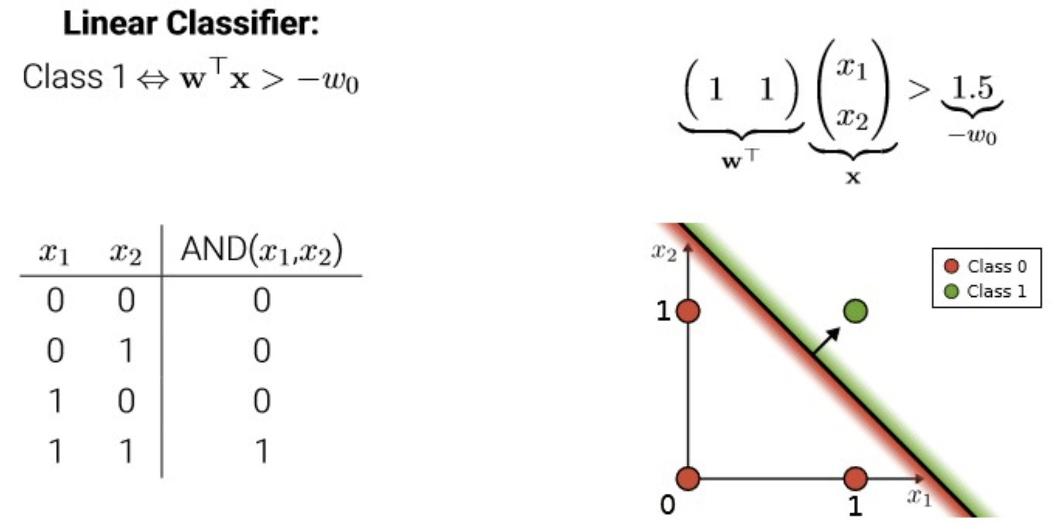
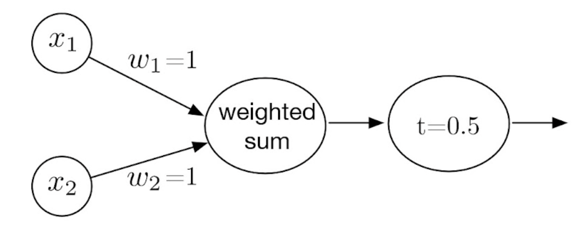
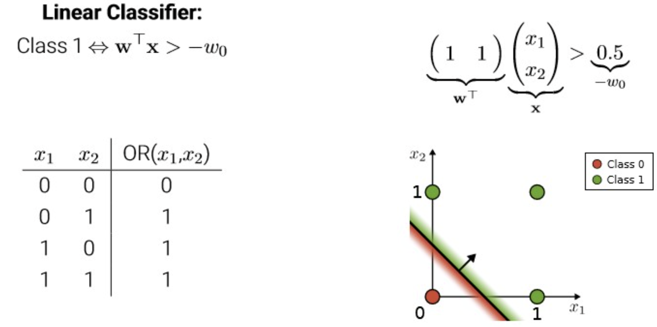
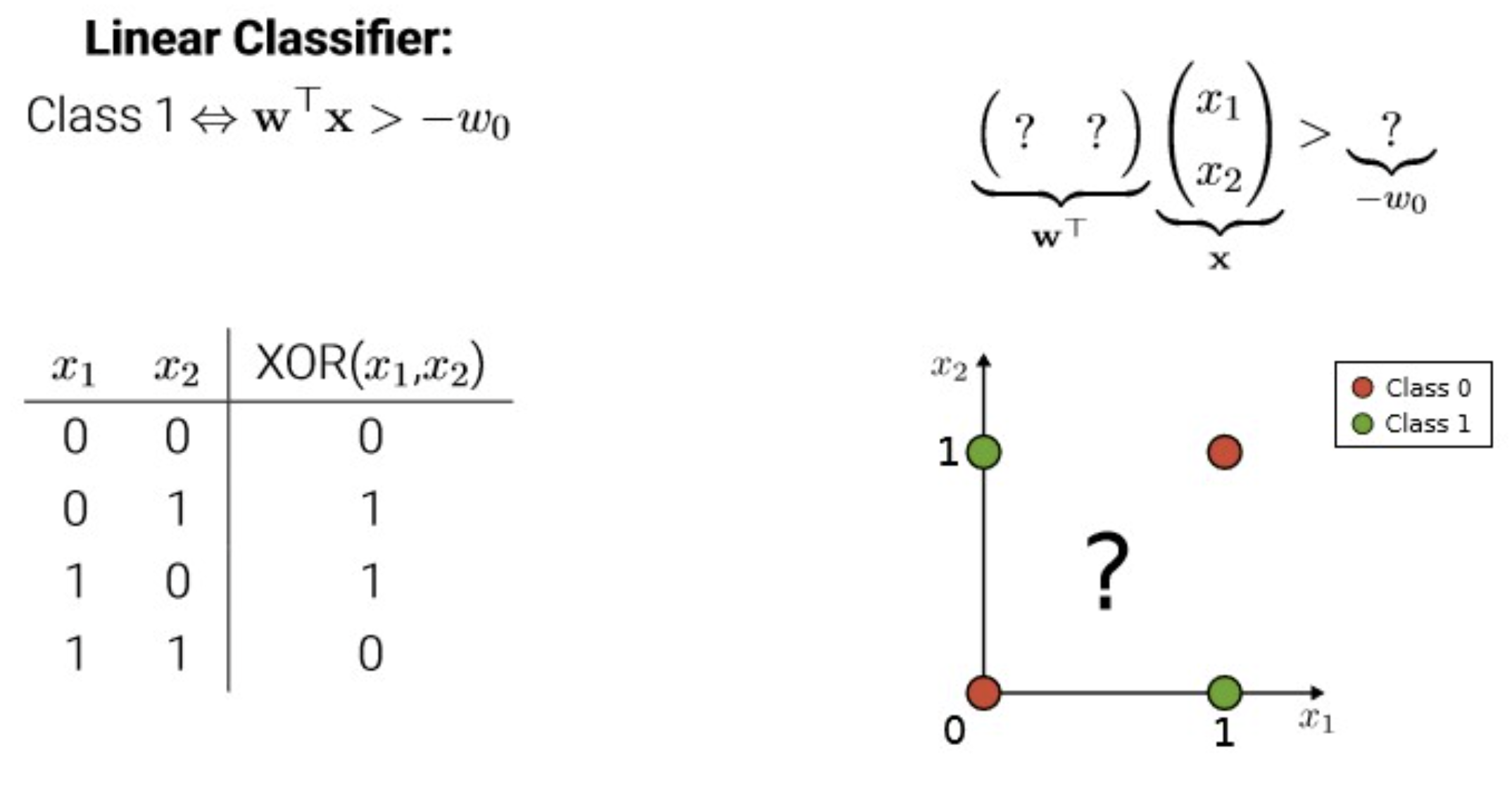
perceptron을 사용하려고 설정하는 것은 여기서 model을 building 하는 단계.

ML as a function approximation

Modeling the relation between input and output using computational components.
How?
→ parameterize the function and learn them from data.

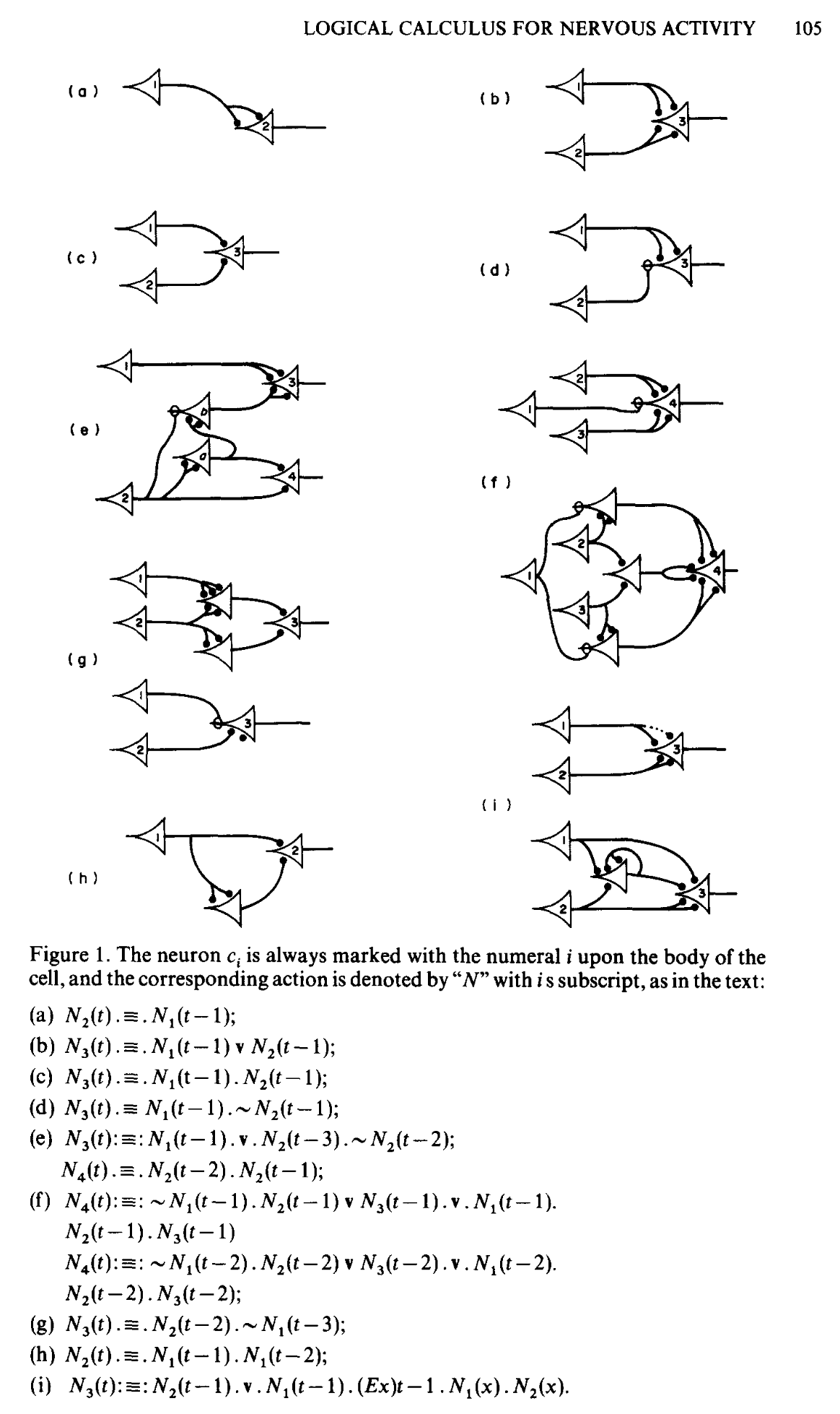
Neuron Model - A logical calculus of the ideas immanet in nervous activity
Abstract

Abstract

Because of the “all-or-none” character of nervous activity, neural events and the relations among them can be treated by means of propositional logic. It is found that the behavior of every net can be described in these terms, with the addition of more complicated logical means for nets containing circles; and that for any logical expression satisfying certain conditions, one can find a net behaving in the fashion it describes. It is shown that many particular choices among possible neurophysiological assumptions are equivalent, in the sense that for every net behaving under one assumption, there exists another net which behaves under the other and gives the same results, although perhaps not in the same time. Various applications of the calculus are discussed.

뉴런의 실무율(0 or 1) 특성을 논리 회로로 볼 수 있지 않을까? 에서 출발하여 이를 구조화 함.

다른 학문들(심리, 신경과학, 뇌 등)에서 다뤄지는 촉진, 억제 등의 활동이 근본적으로 equivalent 하다는 것을 주장.

원본 링크

Perceptron

Perceptron

input들의 weighted sum된 값에 threshold(step-function)을 적용해서 binary 값을 return

Consider a simple model
$\overset{y}{^} = f (x; w, b) = w_{1} x_{1} + w_{2} x_{2} + b$
can be represent as a $\overset{y}{^} = w^{T} x + b$ where $w = [w_{1}, w_{2}]$ and $x = [x_{1}, x_{2}]$ .

이렇게 linear model에서 weighted sum을 계산한 뒤에 threshold값 기준으로 이상인지, 미만인지 판단하여 binary를 return.

Logical AND Gate

Logical AND

Summary

아래와 같은 gate를 만들고 싶은 것.

$x_{1}$ $x_{2}$ $O u t$
0 0 0
0 1 0
1 0 0
1 1 1
이를 모형화 하면,
이렇게 되는데, threshold는 W에 depend.

원본 링크

Logical OR Gate

Logical OR

Summary

아래와 같은 gate를 만들고 싶은 것.

$x_{1}$ $x_{2}$ $O u t$
0 0 0
0 1 1
1 0 1
1 1 1
이를 모형화 하면,
이렇게 되는데, threshold는 W에 depend.

원본 링크

마찬가지로, logical NAND에 대해서도 가능.
NAND = NOT(AND)

XOR problem

XOR problem

Visually, not linearly separable 해보이는데..?

Convex 개념 가져와서 보면,

NOTE

Half spaces(e.g., decision regieon) are convex set.
즉, linear classifier가 나누는 두 영역도 convex set.

NOTE

Suppose there was a feasible hypothesis. If the positive examples are in the positive half-space, then the green line segment must as well.

원본 링크

Convex

Convex

Summary

함수가 아래로 볼록하냐? : convex
위로 볼록(=아래로 오목) : concave

Definition

A set $S$ is convex if any line segment connecting 2 points in $S$ lies entirely within $S$ .
$x_{1}, x_{2} \in S ⟹ λ x_{1} + (1 - λ) x_{2} \in S$ for $λ \in [0, 1]$ .

In the perspective of Optimization…

NOTE

Optimization 관점에서 봤을 때, 함수가 convex 하다면, global minima가 한 개라는 말이니까, GD의 destination이 무조건 global minima 겠지.

원본 링크

MLP

—

이름 그대로 위의 perceptron을 multi-layer 쌓아서 적층한 구조. 각 layer에서 다음 layer로 넘어가는 과정에서 non-linear function을 통과하니, 이때 점차 model에 non-linearity가 생김. 따라서 이러한 구조가 3층이상으로 깊게 쌓이면 Deep-Neural-Network이라 함.

SIMD(Single Instruction Multiple Data)

—

여러 개의 data를 vector 형식으로 묶어서 처리하자!

**

파이썬으로 구현해보기!
Perceptron
class Perceptron():
	def __init__(self, num_features):
		self.num_features = num_features
		self.weights = np.zeros((num_features, 1), dtype=float)
		self.bias = np.zeros(1, dtype=float)
	
	def forward(self, x):
		# $\hat{y} = xw + b$
		linear = np.dot(x, self.weights) + self.bias # comp. net input
		# train에서 보면, y[i] 차원으로 데이터가 들어오니, vec * vec 연산.
		# linear = x @ self.weights + self.bias
		predictions = np.where(linear > 0., 1, 0) # step function - threshold
		return predictions
		
	# 'ppp' exercise
	def backward(self, x, y):
		# pred랑 ground_truth 값 비교.
		return y - self.forward(x)
		
	# 중간 중간 reshape이 과연 필요할까?
	def train(self, x, y, epochs):
		for e in range(epochs):
			for i in range(y.shape[0]):
				errors = self.backward(x[i].reshape(1, self.num_features), y[i]).reshape(-1)
				self.weights += (errors * x[i]).reshape(self.num_features, 1)
				self.bias += errors
	def evaluate(self, x, y):
		predictions = self.forward(x).reshape(-1)
		accuracy = np.sum(predictions == y) / y.shape[0]
		return accuracy
Perceptron-Vectorized version
class Perceptron_vec():
	def __init__(self, num_features):
		self.num_features = num_features
		self.weights = np.zeros((num_features, 1), dtype=float)
		self.bias = np.zeros(1, dtype=float)
		
	def forward(self, x):
		# x: (n, n_features) / weights: (num_features, 1) -> np.dot(x, self.weights) : (n, 1)
		# therefore, self.bias will be broadcasted. self.bias : (1, ) -> (n, )
		# linear : (n, 1) + (n, ) -> (n, 1)
		linear = np.dot(x, self.weights) + self.bias
		# predictions: (n, 1)
		predictions = np.where(linear > 0.5, 1, 0)
		return predictions
		
	def backward(self, x, y):
		# predictions : (n, 1)
		predictions = self.forward(x)
		# errors: (n, 1)
		errors = y - predictions
		return errors
		
	# 'ppp' exercise
	# YOUR CODE HERE
	def train(self, x, y, epochs):
		for e in range(epochs):
			# errors: (n, 1)
			errors = self.backward(x, y.reshape(y.shape[0], 1))
			# self.weights: (n_features, 1)
			# x.T : (n_features, n) / errors: (n, 1)
			self.weights+= np.dot(x.T, errors) # parameter update
			self.bias += errors.mean()
			
	def evaluate(self, x, y):
		predictions = self.forward(x).reshape(-1)
		accuracy = np.sum(predictions == y) / y.shape[0]
		return accuracy
Training Code
ppn = Perceptron(num_features = 2)
 
pp.train(X_train, y_train, epochs=5)
 
print('Model parameters:\n\n')
print('Weights: %s\n ' % ppn.weights)
print('Bias: %s\n ' % ppn.bias)
Evaluating Code
train_acc = ppn.evaluate(X_train, y_train)
print('Train set accuracy: %.2f ' % (test_acc*100))
Decision Boundary plot
##########################
### 2D Decision Boundary
##########################
w, b = ppn.weights, ppn.bias
 
x0_min = -2
x1_min = ((-(w[0] * x0_min) - b[0]) / w[1])
 
x0_max = 2
x1_max = ((-(w[0] * x0_max) - b[0]) / w[1])
 
# x0*w0 + x1*w1 + b = 0
# x1 = (-x0*w0 - b) / w1
# 'ppp' exercise
 
import matplotlib.pyplot as plt
fig, ax = plt.subplots(nrows=1, ncols=2, sharex = True, figsize=(10, 5))
 
for idx, ax_i in enumerate(ax):
	ax_i.plot([x0_min, x0_max], [x1_min, x1_max]) # decision boundary
	ax_i.set_xlabel('feature 1')
	ax_i.set_ylabel('feature 2')
	ax_i.set_xlim([-3, 3])
	ax_i.set_ylim([-3, 3])
	
	if idx == 0:
		ax_i.set_title('Training set')
		ax_i.scatter(X_train[y_train==0, 0], X_train[y_train==0, 1], label='class 0', marker='o')
		ax_i.scatter(X_train[y_train==1, 0], X_train[y_train==1, 1], label='class 1', marker='s')
	else:
		ax_i.set_title('Test set')
		ax_i.scatter(X_test[y_test==0, 0], X_test[y_test==0, 1], label='class 0', marker='o')
		ax_i.scatter(X_test[y_test==1, 0], X_test[y_test==1, 1], label='class 1', marker='s')
		
	ax_i.legend(loc='upper left')
	plt.show()
원본 링크

Juhyeon's Blog

탐색기

RR02. Preliminaries -2

Neuron Model - A logical calculus of the ideas immanet in nervous activity

Abstract

Perceptron

Logical AND Gate

Logical AND

Logical OR Gate

Logical OR

XOR problem

XOR problem

Convex

Convex

Definition

In the perspective of Optimization…

그래프 뷰

Properties

백링크

$x_{1}$	$x_{2}$	$O u t$
0	0	0
0	1	0
1	0	0
1	1	1
이를 모형화 하면,

이렇게 되는데, threshold는 W에 depend.