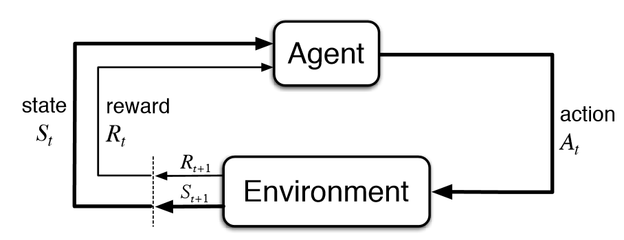
Reward 라고 하는 값을 long-term으로 봤을 때 maximize 하도록 function을 학습하는 기법이다.
기본적인 paradigm은 Env(환경)에 Agent를 넣고 둘 간의 interaction을 보는 것이다.
주고 받는 정보는 아래와 같으며, agent가 action을 함으로써 state가 transition되고, env로부터 reward가 계산되며 계속 action을 하는 방향으로 학습된다.
ex) games, Go, chess, etc…
Important
long-term의 reward를 극대화하는 것이 목표이므로, 단기적 손실은 희생(sacrifice)한다.
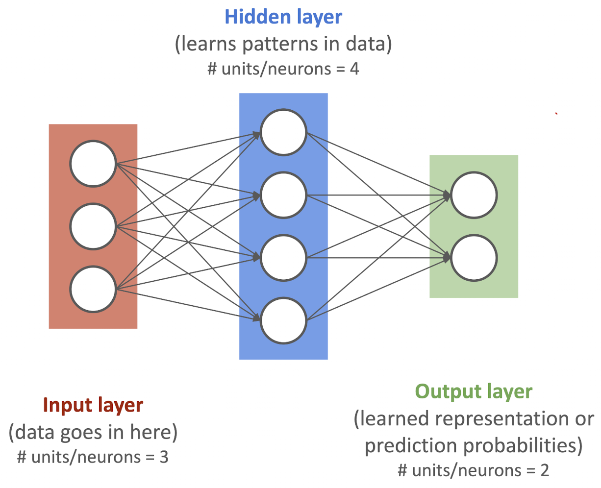
Note1. 각 Layer는 linear / non-linear function들오 연결되어 있다. Note 2. “pattern” == “embedding”, “weights”, “feature representation”, “feature vectors” 다 비슷한 걸 가르킨다. ! Note 3 !. layer의 개수를 셀 때에는 input-layer는 제외한다.
Why Do We Need Non-linearity?
Non-Linearity
Nonlinearity
복잡한 현실 세계의 복잡한 함수를 다루기 위해
matrix의 matmul이 결국 linear하니까, non-linear 함수를 중간에 끼지 않는 이상 결국은 하나의 큰 선형 시스템을 벗어날 수 없음. 세상이 선형함수로만 설명 가능할리 없잖아,,
→ 선형 연산을 거듭해도 선형.
Numerical Proof
Assume that,
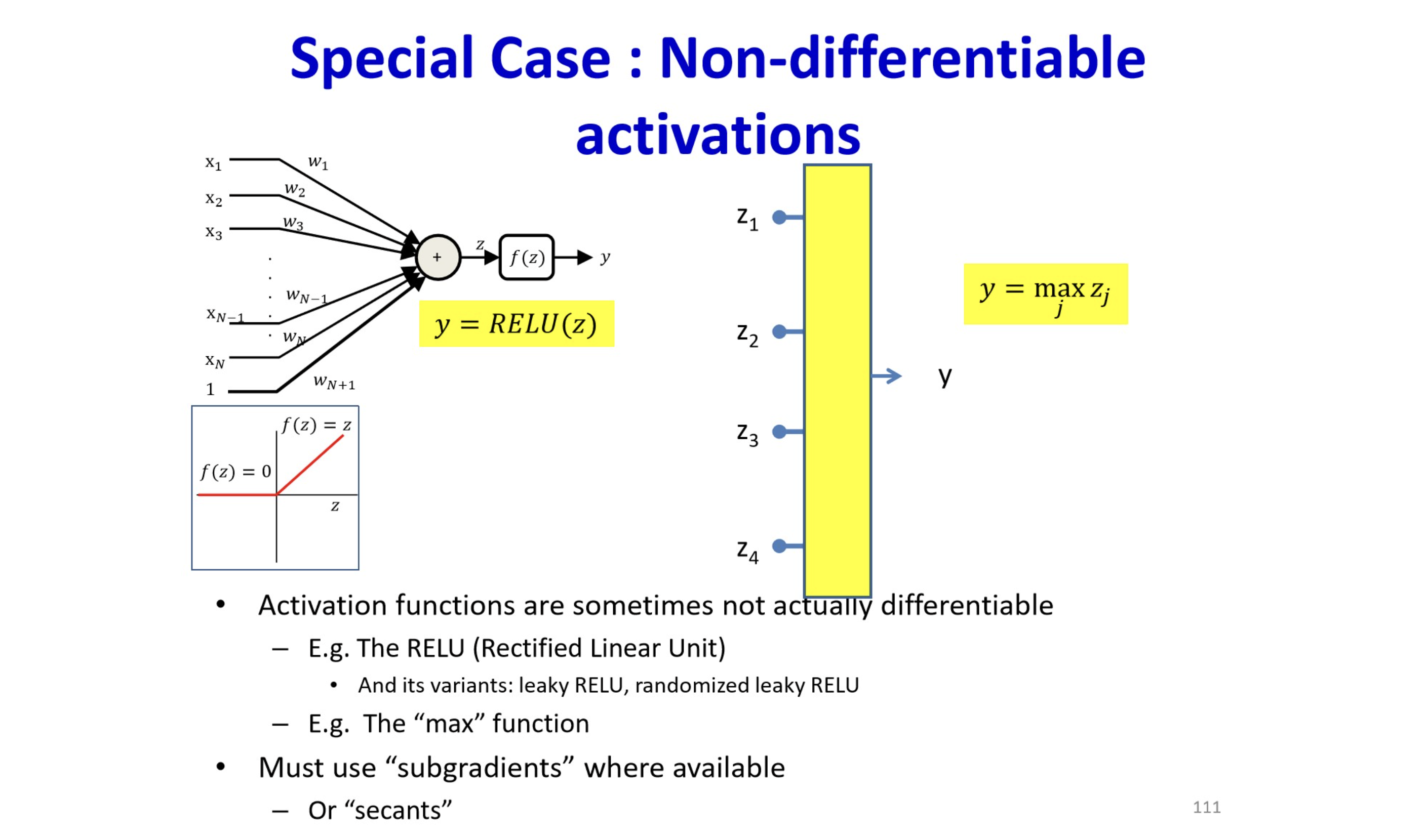
f=W2⋅max(0,W1⋅x)
where x∈RD, W1∈RH×D, W2∈RC×H
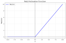
ReLU
ReLU(x)=max(0,x)
one of non-linear activation
In this time, it is impossible to distinguish below 2 models,
f=W2⋅W1⋅x f=W3⋅x
where W3∈RC×H
→ 결국 linear
→ 그러니 non-linear function을 activation으로 사용하자!!
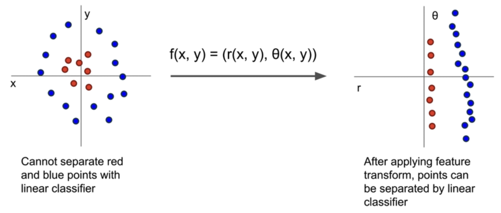
Linearly Separable ← 고민 좀 해보자. 왜 좋냐?
Important
non-linear map은 data를 linearly-separable하게 바꿀 수 있다.
Examples
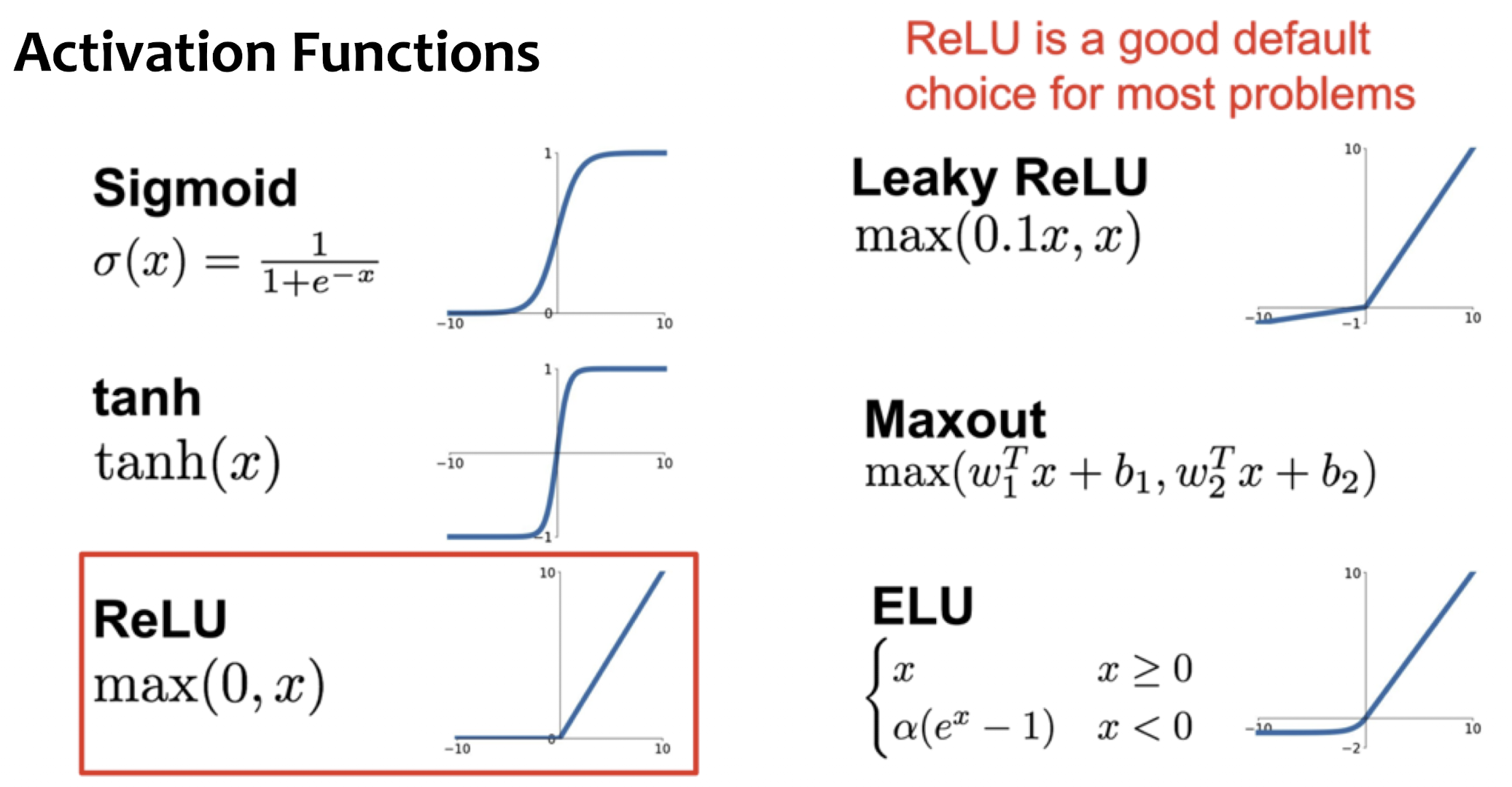
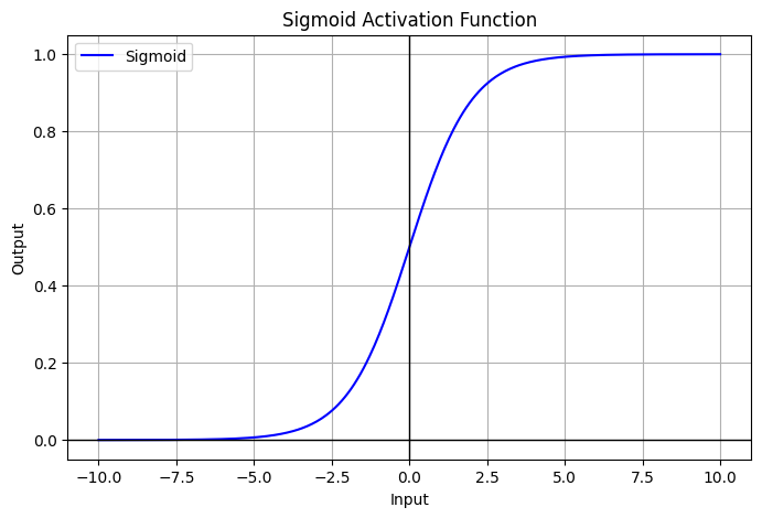
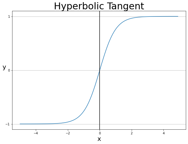
Activation Functions
나중에 transformer 계열에 최근 가장 많이 사용되는 GeLU 계열이나 찾아볼 것.
Summary
No one-size-fits-all: Choice of activation function depends on problem.
We only showed the most common ones, there exist many more
Best activation function / model is often using trial-and-error in practice
It is important to ensure a good “gradient flow” during optimization
Rule of Thumb
Use ReLU by default(with small enough lr)
Try Leaky ReLU, Maxout, ELU for some small additional gain
Prefer Tanh over sigmoid(Tanh often used in RNNs)
ReLU
ReLU(Rectified Linear Unit)
activation 중 하나로 대표적으로 많이 사용됨. g(x)=max(x,0)
Does not saturate(for x>0)
Leads to fast convergence
Computationally efficient
Problems
No learning for x<0 → dead/dying ReLU
downstream gradient가 0(input이 0 이하일 때,)
often initialize with pos. bias (b>0)
Outputs are not zero-centered → introduces bias after the layer
sigmoid와 그 gradient는 항상 positive이기 때문에 model wight의 bias
작은 loss는 generalization 성능을 말해주는 게 아닌, 단순 train-set에 대한 explainability를 말해주니,
모델 구조, 데이터 셋, optimization method 등에 따라 값 자체가 너무 달라지니, 일관성있는 비교가 힘듦.
아래는 대표적인 evaluation metric이다.
For Regression
Important
Regression task에서, ground true(label)는 floating point value 즉, prediction value는 저 값 자체에 가까워지는 것이 목표이므로, loss 자체가 evaluation metric으로써의 기능도 할 수 있다. 따라서 아래에 있는 Mean Square Error(MSE), Mean Absolute Error(MAE) 같은 경우는 loss 임과 동시에 evaluation metric의 기능도 할 수 있다.
다만, 꼭 같은 값을 evaluation metric으로 사용할 필요는 없으나, 학습하는 과정에서 사용한 loss와 metric이 일치할 경우에는 loss 가 줄어드는 정보만으로 evaluation value도 감소할 것이라 추정할 수는 있겠지.
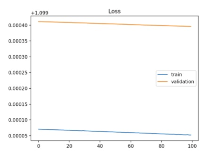
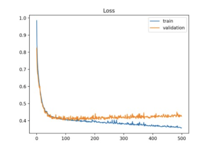
Training loss는 계속 줄지만, validation loss은 낮아지지 않음.
train을 계속하면, 모델은 train-set에만 잘 작동하는 함수로 fitting되니,
generalization이 떨어지고, validation-set 또는 unseen-data에 대해서도 loss가 커짐.
Help
To solve the problem, several methods are recommended.
Get more data: 사실상 이게 best. 그러나 cost-issue.
모델한테 패턴을 학습할 기회를 더 주는 것.
Data Augmentation : 데이터를 더 collecting 하는 것 보단 현실적.
train-set의 diversity를 주는 것.
Better Data: low-quality data를 remove.
Transfer Learning: task-suit 하게 준비된 set으로 fine-tune.
Simplify model: 모델의 capacity가 충분해서 train-set의 너무 과한 패턴을 학습한 거니, 모델의 복잡성을 줄여서 generalization performance 확보.
Learning Rate decay: fine-tune은 학습 후반에서 미세한 gradient에서 학습하는 거니, decaying은 후반에서 이러한 것들을 완화해줌.